Statistics for Decision Making

This article discusses statistics for decision making, covering questionnaire method, convenience sampling, numerical summary, regression analysis, and more. The article also includes a table of numerical summary, scatter plot, regression summary table, and hypothesis testing. The dependent variable is weekly television watching hours and the independent variable is the total debt for each family. The article concludes with a discussion on the adverse effect of TV hours on the financial situation of the family and the need to collect information about other factors affecting total debt.

Statistics for Decision Making

Part 1
a) The researcher could have used Questionnaire method to do the survey. Questionnaire
method would have been cost effective and convenient to collect data from large number
of respondents compared to interview method.
b) Convenience sampling could have been used by the researcher. This type of survey helps
to collect data on a particular topic from a selected segment of people. Researcher
collected data from the population about television watching hours and family debts.
Information about these particular variables could have been collected from a particular
segment of the society.
c) Other than the present two variables, information regarding age, gender, income, and
number of family members of the respondents should be collected. Age and gender could
facilitate the researcher with a gender based or age based cross sectional study.
d) Age is a continuous ratio (scale) variable, gender is a nominal variable; income is a
continuous interval (scale) variable, number of family members is discrete variable.
Television hours is a continuous interval variable, and debt is a continuous interval
(scale) variable.
e) For convenience sampling method the sample was collected from a particular group, and
could have been biased. The researcher might not obtain a generalized result from the
analysis.

Part 2
a) The researcher probably could have used Struge formula to determine number of classes
as C=1+3 .222 log N=1+3 . 222*log 400=1+3. 222∗2. 6020=1+8 . 38≃10 where N was the
number of observations (Rodarte, Carmona, and Rodríguez, 2016). Such formula is used
to make the classes equally spaced.
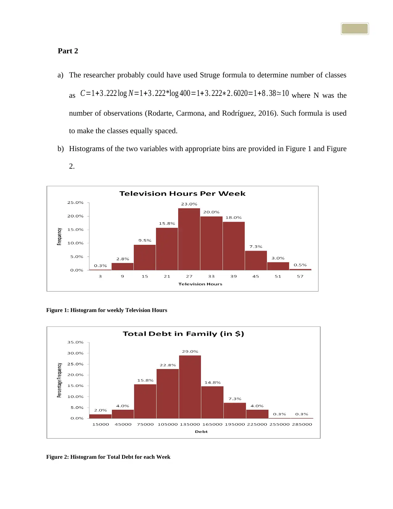
b) Histograms of the two variables with appropriate bins are provided in Figure 1 and Figure
2.
Figure 1: Histogram for weekly Television Hours
Figure 2: Histogram for Total Debt for each Week

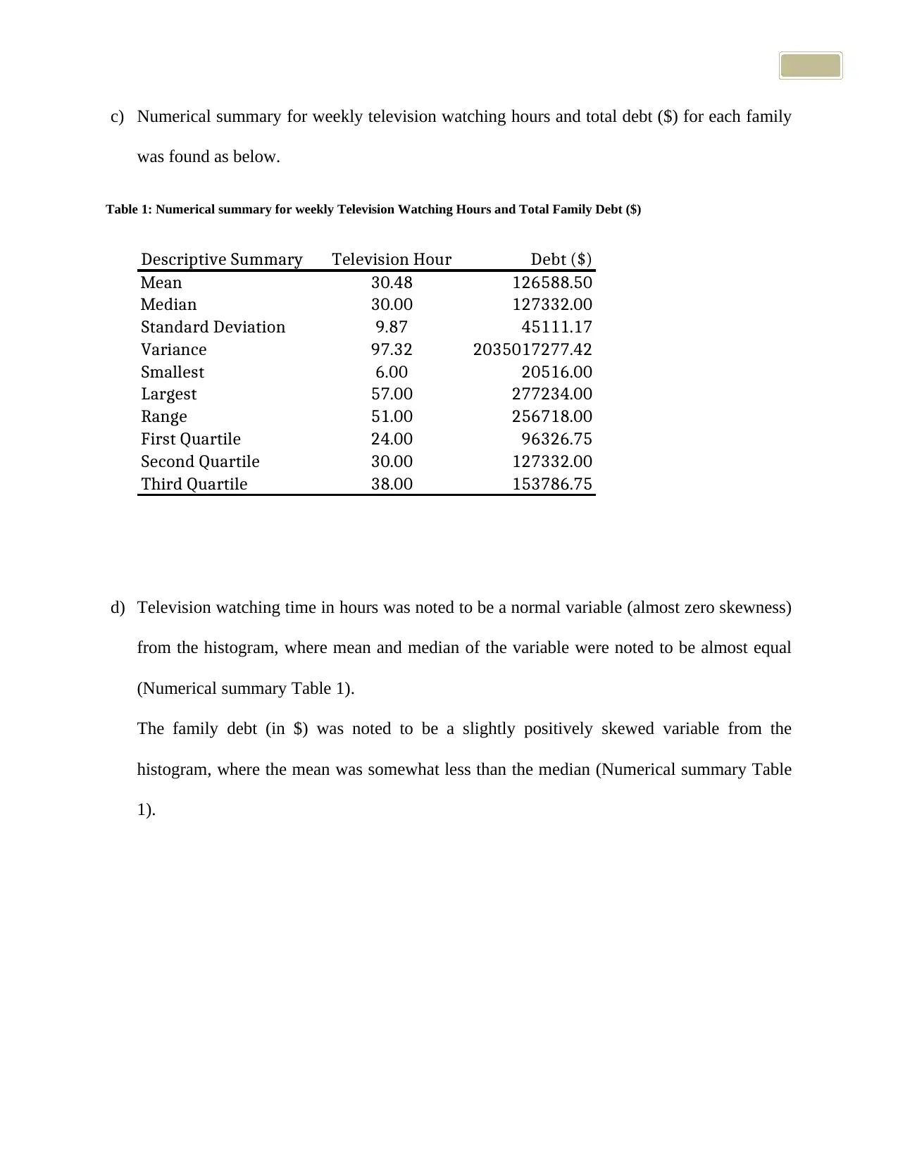
c) Numerical summary for weekly television watching hours and total debt ($) for each family
was found as below.
Table 1: Numerical summary for weekly Television Watching Hours and Total Family Debt ($)
Descriptive Summary Television Hour Debt ($)
Mean 30.48 126588.50
Median 30.00 127332.00
Standard Deviation 9.87 45111.17
Variance 97.32 2035017277.42
Smallest 6.00 20516.00
Largest 57.00 277234.00
Range 51.00 256718.00
First Quartile 24.00 96326.75
Second Quartile 30.00 127332.00
Third Quartile 38.00 153786.75
d) Television watching time in hours was noted to be a normal variable (almost zero skewness)
from the histogram, where mean and median of the variable were noted to be almost equal
(Numerical summary Table 1).
The family debt (in $) was noted to be a slightly positively skewed variable from the
histogram, where the mean was somewhat less than the median (Numerical summary Table
1).

Part 3
a) The dependent variable could be weekly television watching hours (Y) and independent
variable could be the total debt ($) for each family (X).
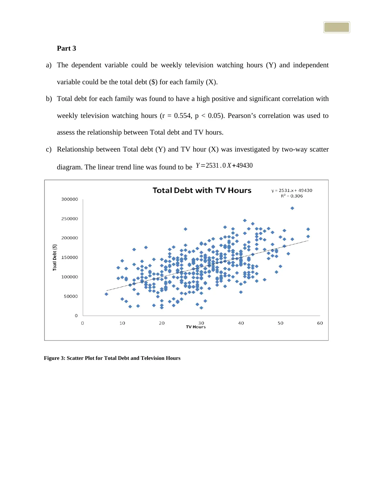
b) Total debt for each family was found to have a high positive and significant correlation with
weekly television watching hours (r = 0.554, p < 0.05). Pearson’s correlation was used to
assess the relationship between Total debt and TV hours.
c) Relationship between Total debt (Y) and TV hour (X) was investigated by two-way scatter
diagram. The linear trend line was found to be Y =2531 . 0 X +49430
Figure 3: Scatter Plot for Total Debt and Television Hours

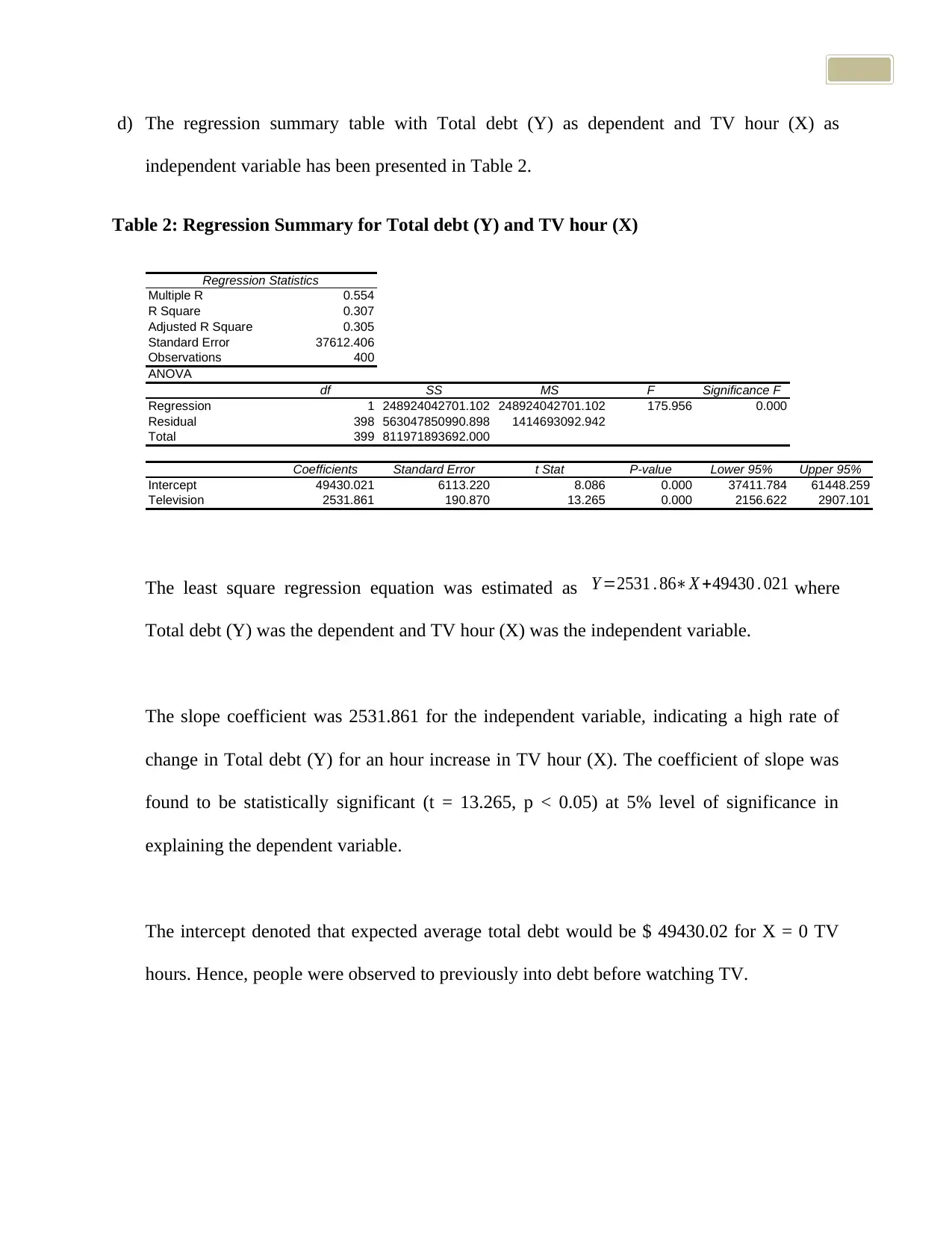
d) The regression summary table with Total debt (Y) as dependent and TV hour (X) as
independent variable has been presented in Table 2.
Table 2: Regression Summary for Total debt (Y) and TV hour (X)
Regression Statistics
Multiple R 0.554
R Square 0.307
Adjusted R Square 0.305
Standard Error 37612.406
Observations 400
ANOVA
df SS MS F Significance F
Regression 1 248924042701.102 248924042701.102 175.956 0.000
Residual 398 563047850990.898 1414693092.942
Total 399 811971893692.000
Coefficients Standard Error t Stat P-value Lower 95% Upper 95%
Intercept 49430.021 6113.220 8.086 0.000 37411.784 61448.259
Television 2531.861 190.870 13.265 0.000 2156.622 2907.101
The least square regression equation was estimated as Y =2531 . 86∗X +49430 . 021 where
Total debt (Y) was the dependent and TV hour (X) was the independent variable.
The slope coefficient was 2531.861 for the independent variable, indicating a high rate of
change in Total debt (Y) for an hour increase in TV hour (X). The coefficient of slope was
found to be statistically significant (t = 13.265, p < 0.05) at 5% level of significance in
explaining the dependent variable.
The intercept denoted that expected average total debt would be $ 49430.02 for X = 0 TV
hours. Hence, people were observed to previously into debt before watching TV.

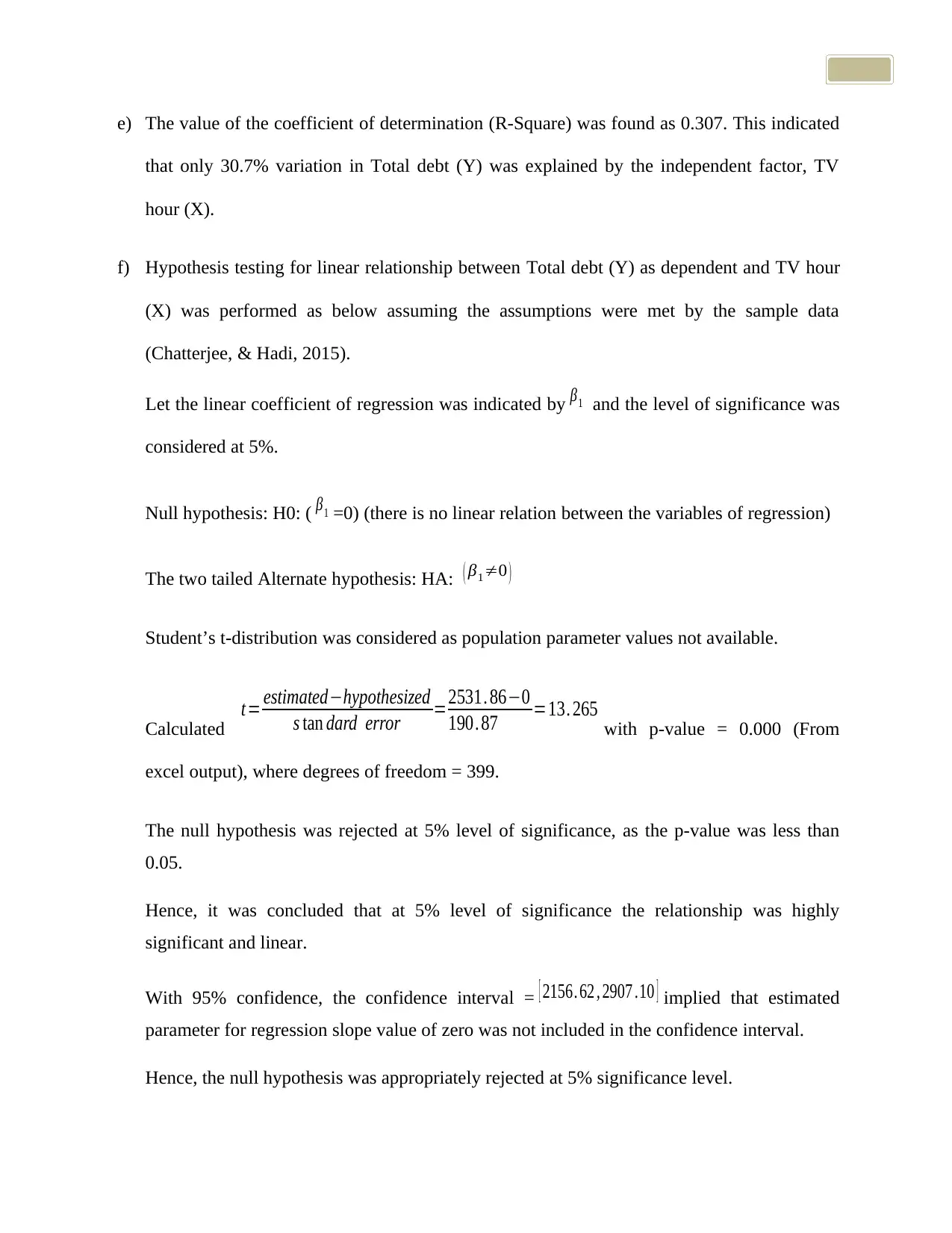
e) The value of the coefficient of determination (R-Square) was found as 0.307. This indicated
that only 30.7% variation in Total debt (Y) was explained by the independent factor, TV
hour (X).
f) Hypothesis testing for linear relationship between Total debt (Y) as dependent and TV hour
(X) was performed as below assuming the assumptions were met by the sample data
(Chatterjee, & Hadi, 2015).
Let the linear coefficient of regression was indicated by β1 and the level of significance was
considered at 5%.
Null hypothesis: H0: ( β1 =0) (there is no linear relation between the variables of regression)
The two tailed Alternate hypothesis: HA: ( β1≠0 )
Student’s t-distribution was considered as population parameter values not available.
Calculated
t= estimated−hypothesized
s tan dard error =2531. 86−0
190. 87 =13. 265 with p-value = 0.000 (From
excel output), where degrees of freedom = 399.
The null hypothesis was rejected at 5% level of significance, as the p-value was less than
0.05.
Hence, it was concluded that at 5% level of significance the relationship was highly
significant and linear.
With 95% confidence, the confidence interval = [ 2156. 62 , 2907 .10 ] implied that estimated
parameter for regression slope value of zero was not included in the confidence interval.
Hence, the null hypothesis was appropriately rejected at 5% significance level.

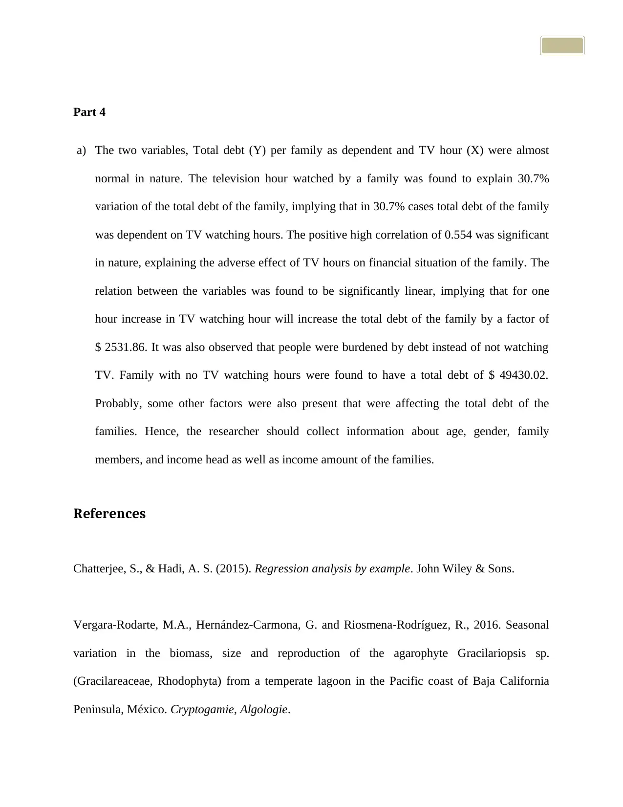
Part 4
a) The two variables, Total debt (Y) per family as dependent and TV hour (X) were almost
normal in nature. The television hour watched by a family was found to explain 30.7%
variation of the total debt of the family, implying that in 30.7% cases total debt of the family
was dependent on TV watching hours. The positive high correlation of 0.554 was significant
in nature, explaining the adverse effect of TV hours on financial situation of the family. The
relation between the variables was found to be significantly linear, implying that for one
hour increase in TV watching hour will increase the total debt of the family by a factor of
$ 2531.86. It was also observed that people were burdened by debt instead of not watching
TV. Family with no TV watching hours were found to have a total debt of $ 49430.02.
Probably, some other factors were also present that were affecting the total debt of the
families. Hence, the researcher should collect information about age, gender, family
members, and income head as well as income amount of the families.
References
Chatterjee, S., & Hadi, A. S. (2015). Regression analysis by example. John Wiley & Sons.
Vergara-Rodarte, M.A., Hernández-Carmona, G. and Riosmena-Rodríguez, R., 2016. Seasonal
variation in the biomass, size and reproduction of the agarophyte Gracilariopsis sp.
(Gracilareaceae, Rhodophyta) from a temperate lagoon in the Pacific coast of Baja California
Peninsula, México. Cryptogamie, Algologie.