MATH221 Statistics for Decision Making: Week 6 Lab Assignment Analysis
VerifiedAdded on 2022/09/27
|9
|1334
|24
Homework Assignment
AI Summary
This assignment provides a comprehensive solution to a Week 6 lab in a Statistics for Decision Making course (MATH221), focusing on statistical concepts such as confidence intervals, data simulation, and normal probabilities. The solution begins by calculating and interpreting 95% and 99% confidence intervals for the sleep variable, separated by gender, and compares the results. It then proceeds to calculate and interpret confidence intervals for shoe size, comparing the 95% and 99% intervals and explaining the differences. Finally, the assignment analyzes the DRIVE variable, predicting and calculating percentages of data points within specific ranges, comparing these predictions to actual data, and explaining any discrepancies based on the distribution of the data. The solution incorporates the use of spreadsheets for calculations and includes references to supporting statistical literature.
MATH221 Statistics for Decision Making
Week 6 Lab
Name: _______________________
Statistical Concepts:
Confidence Intervals
Data Simulation
Normal Probabilities
Short Answer Writing Assignment
All answers should be complete sentences.
In the Week 2 Lab, you found the mean and the standard deviation for the SLEEP
variable for both males and females. Use those values for follow these directions to
calculate the numbers again.
(From Week 2 Lab: Calculate descriptive statistics for the variable Sleep by Gender.
Sort the data by gender by clicking on Data and then Sort. Copy the Sleep of the
males from the data file into the Descriptive Statistics worksheet of the Week 1 Excel
file. [Write down the mean and standard deviation.] These are sample data. Then,
Paraphrase This Document
Need a fresh take? Get an instant paraphrase of this document with our AI Paraphraser
copy and paste the female data into the Descriptive Statistics workbook and do the
same. Keep three decimal places.)
You will also need the number of males and the number of females in the dataset. You
can actually count these in the dataset.
Then use the Week 5 spreadsheet to calculate the following confidence intervals. The
male confidence interval would be one calculation in the spreadsheet and the females
would be a second calculation.
Solution
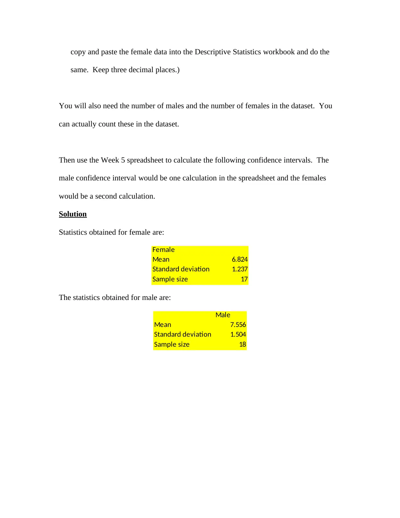
Statistics obtained for female are:
Female
Mean 6.824
Standard deviation 1.237
Sample size 17
The statistics obtained for male are:
Male
Mean 7.556
Standard deviation 1.504
Sample size 18
same. Keep three decimal places.)
You will also need the number of males and the number of females in the dataset. You
can actually count these in the dataset.
Then use the Week 5 spreadsheet to calculate the following confidence intervals. The
male confidence interval would be one calculation in the spreadsheet and the females
would be a second calculation.
Solution
Statistics obtained for female are:
Female
Mean 6.824
Standard deviation 1.237
Sample size 17
The statistics obtained for male are:
Male
Mean 7.556
Standard deviation 1.504
Sample size 18
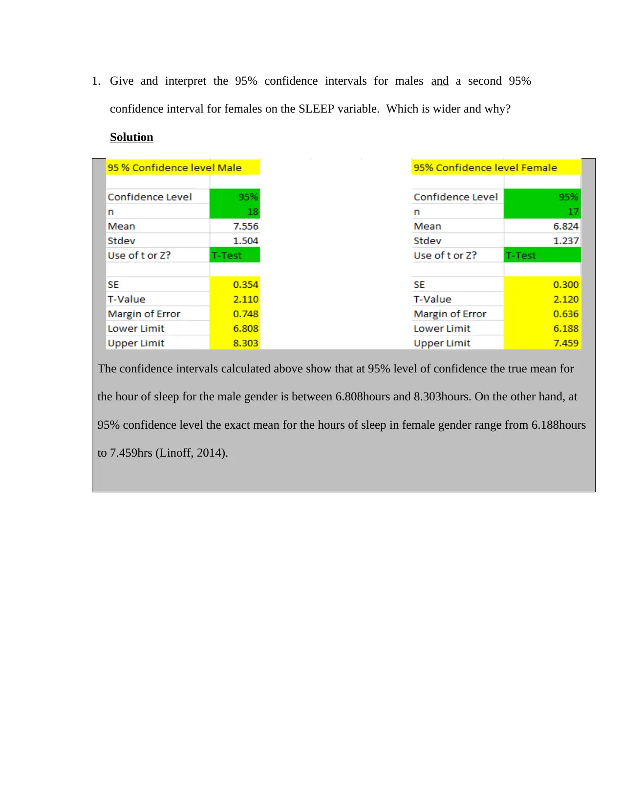
1. Give and interpret the 95% confidence intervals for males and a second 95%
confidence interval for females on the SLEEP variable. Which is wider and why?
Solution
The confidence intervals calculated above show that at 95% level of confidence the true mean for
the hour of sleep for the male gender is between 6.808hours and 8.303hours. On the other hand, at
95% confidence level the exact mean for the hours of sleep in female gender range from 6.188hours
to 7.459hrs (Linoff, 2014).
⊘ This is a preview!⊘
Do you want full access?
Subscribe today to unlock all pages.
Trusted by 1+ million students worldwide
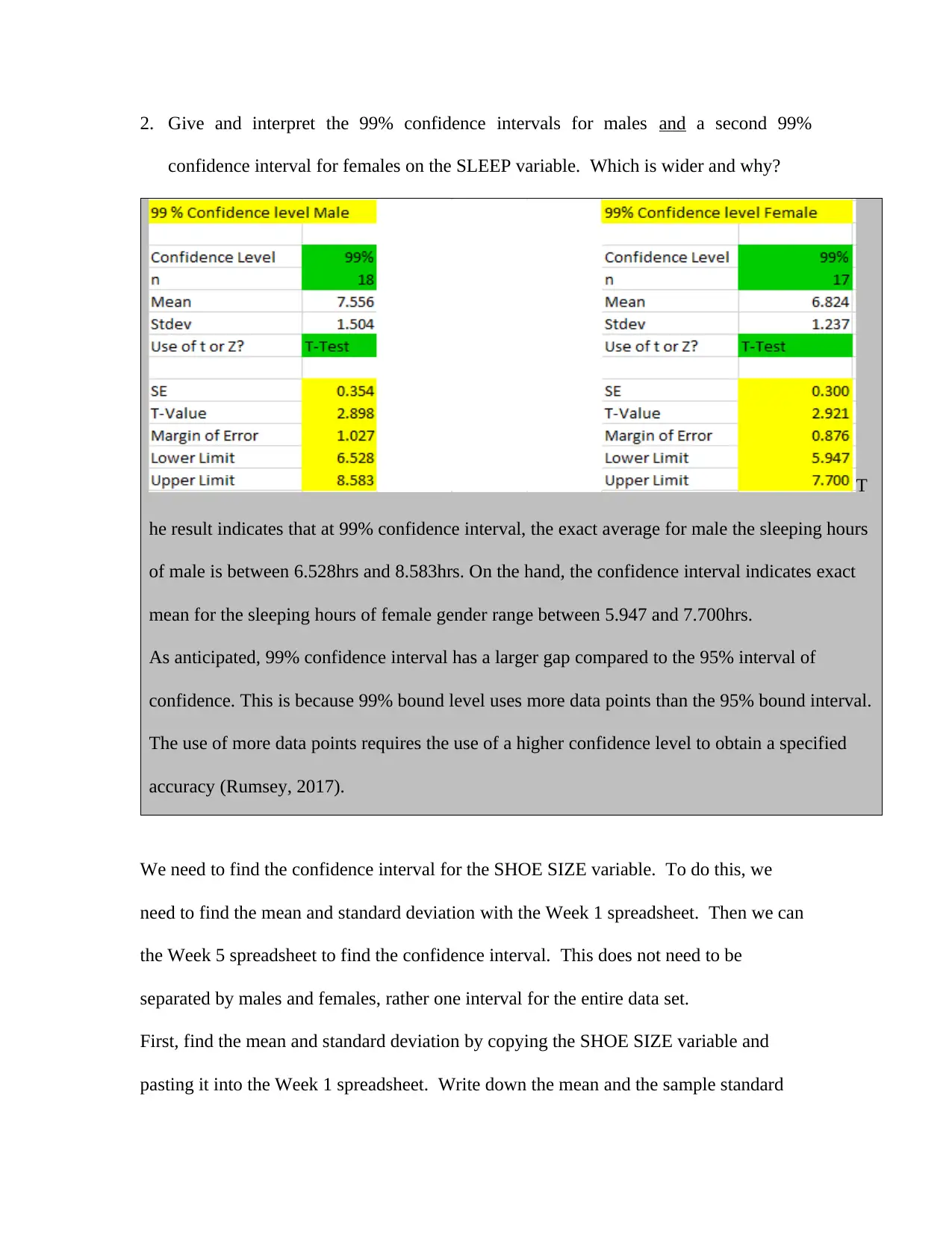
2. Give and interpret the 99% confidence intervals for males and a second 99%
confidence interval for females on the SLEEP variable. Which is wider and why?
T
he result indicates that at 99% confidence interval, the exact average for male the sleeping hours
of male is between 6.528hrs and 8.583hrs. On the hand, the confidence interval indicates exact
mean for the sleeping hours of female gender range between 5.947 and 7.700hrs.
As anticipated, 99% confidence interval has a larger gap compared to the 95% interval of
confidence. This is because 99% bound level uses more data points than the 95% bound interval.
The use of more data points requires the use of a higher confidence level to obtain a specified
accuracy (Rumsey, 2017).
We need to find the confidence interval for the SHOE SIZE variable. To do this, we
need to find the mean and standard deviation with the Week 1 spreadsheet. Then we can
the Week 5 spreadsheet to find the confidence interval. This does not need to be
separated by males and females, rather one interval for the entire data set.
First, find the mean and standard deviation by copying the SHOE SIZE variable and
pasting it into the Week 1 spreadsheet. Write down the mean and the sample standard
Paraphrase This Document
Need a fresh take? Get an instant paraphrase of this document with our AI Paraphraser
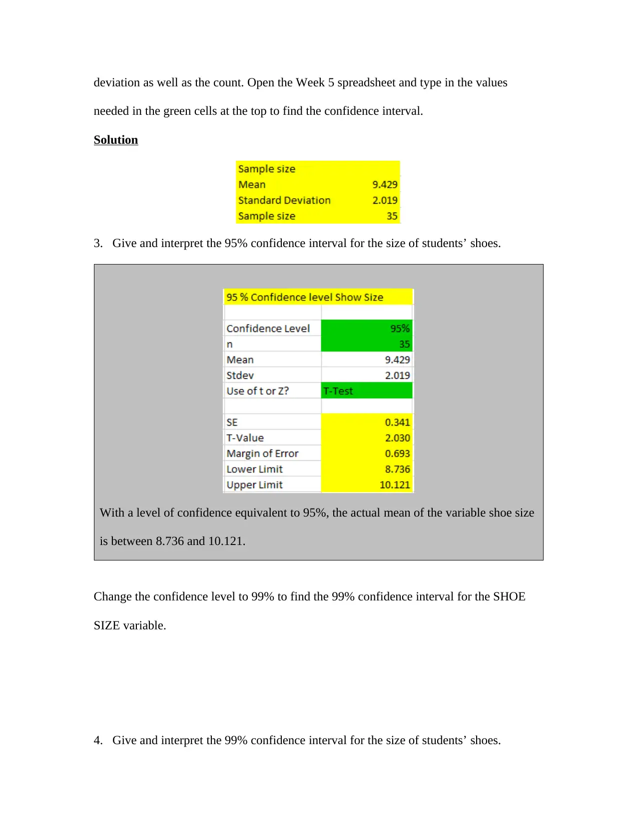
deviation as well as the count. Open the Week 5 spreadsheet and type in the values
needed in the green cells at the top to find the confidence interval.
Solution
3. Give and interpret the 95% confidence interval for the size of students’ shoes.
With a level of confidence equivalent to 95%, the actual mean of the variable shoe size
is between 8.736 and 10.121.
Change the confidence level to 99% to find the 99% confidence interval for the SHOE
SIZE variable.
4. Give and interpret the 99% confidence interval for the size of students’ shoes.
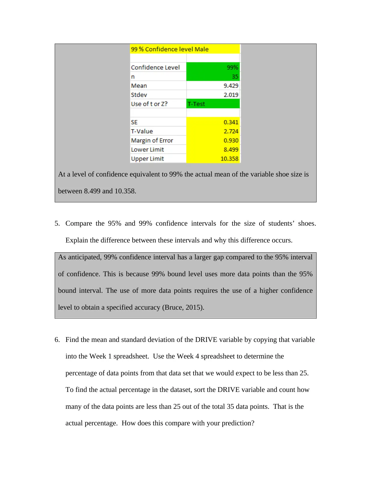
At a level of confidence equivalent to 99% the actual mean of the variable shoe size is
between 8.499 and 10.358.
5. Compare the 95% and 99% confidence intervals for the size of students’ shoes.
Explain the difference between these intervals and why this difference occurs.
As anticipated, 99% confidence interval has a larger gap compared to the 95% interval
of confidence. This is because 99% bound level uses more data points than the 95%
bound interval. The use of more data points requires the use of a higher confidence
level to obtain a specified accuracy (Bruce, 2015).
6. Find the mean and standard deviation of the DRIVE variable by copying that variable
into the Week 1 spreadsheet. Use the Week 4 spreadsheet to determine the
percentage of data points from that data set that we would expect to be less than 25.
To find the actual percentage in the dataset, sort the DRIVE variable and count how
many of the data points are less than 25 out of the total 35 data points. That is the
actual percentage. How does this compare with your prediction?
⊘ This is a preview!⊘
Do you want full access?
Subscribe today to unlock all pages.
Trusted by 1+ million students worldwide
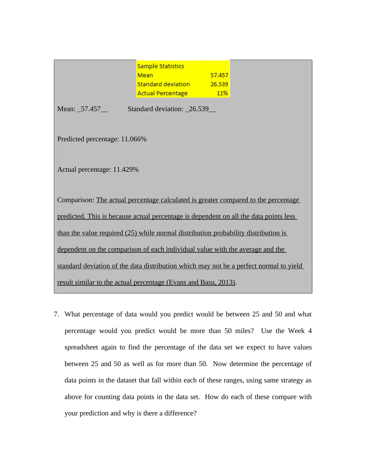
Mean: _57.457__ Standard deviation: _26.539__
Predicted percentage: 11.066%
Actual percentage: 11.429%
Comparison: The actual percentage calculated is greater compared to the percentage
predicted. This is because actual percentage is dependent on all the data points less
than the value required (25) while normal distribution probability distribution is
dependent on the comparison of each individual value with the average and the
standard deviation of the data distribution which may not be a perfect normal to yield
result similar to the actual percentage (Evans and Basu, 2013).
7. What percentage of data would you predict would be between 25 and 50 and what
percentage would you predict would be more than 50 miles? Use the Week 4
spreadsheet again to find the percentage of the data set we expect to have values
between 25 and 50 as well as for more than 50. Now determine the percentage of
data points in the dataset that fall within each of these ranges, using same strategy as
above for counting data points in the data set. How do each of these compare with
your prediction and why is there a difference?
Paraphrase This Document
Need a fresh take? Get an instant paraphrase of this document with our AI Paraphraser
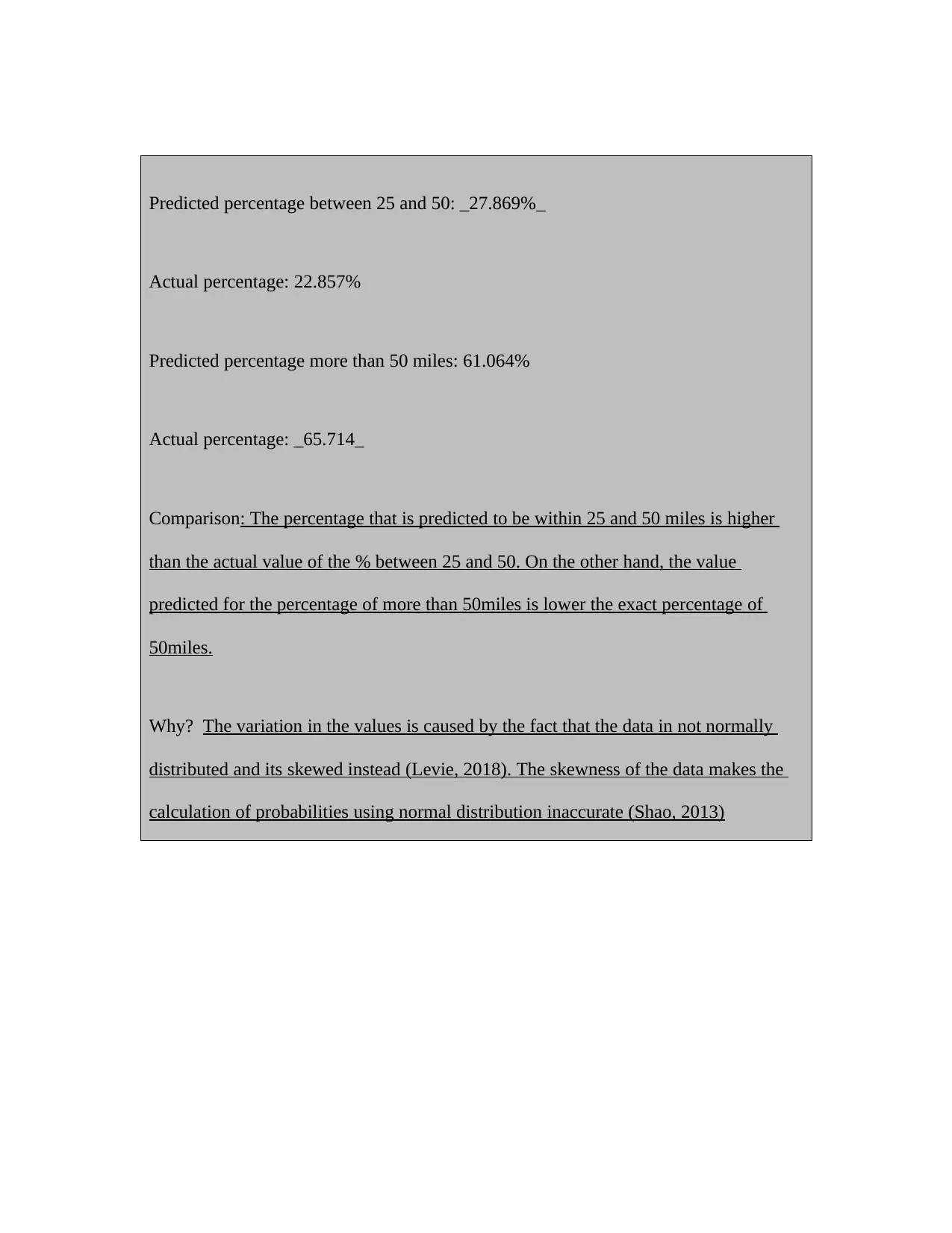
Predicted percentage between 25 and 50: _27.869%_
Actual percentage: 22.857%
Predicted percentage more than 50 miles: 61.064%
Actual percentage: _65.714_
Comparison: The percentage that is predicted to be within 25 and 50 miles is higher
than the actual value of the % between 25 and 50. On the other hand, the value
predicted for the percentage of more than 50miles is lower the exact percentage of
50miles.
Why? The variation in the values is caused by the fact that the data in not normally
distributed and its skewed instead (Levie, 2018). The skewness of the data makes the
calculation of probabilities using normal distribution inaccurate (Shao, 2013)
References
Bruce, P. 2015. Introductory statistics and analytics. New Jersey: Wiley.
Evans, J. R., and Basu, A. 2013. Statistics, data analysis, and decision modeling.5th ed.
Boston: Pearson.
Levie, R. D. 2018. Advanced Excel for scientific data analysis. 2nd ed. New York, NY:
Oxford University Press.
Linoff, G. 2014. Data analysis using SQL and Excel. Indianapolis, Ind.: Wiley Pub.
Rumsey, D. 2017. Intermediate statistics for dummies. 3rd ed. Hoboken, N.J.: Wiley
Shao, J. 2013. Mathematical statistics. 2nd ed. New York: Springer.
⊘ This is a preview!⊘
Do you want full access?
Subscribe today to unlock all pages.
Trusted by 1+ million students worldwide
1 out of 9