Employee Earnings Analysis and Recommendations

This assignment involves analyzing employee earnings data presented in an ogive chart. The task is to identify trends, recommend salary increases for the 20-25 range, decreases for those under 10, and suggest adopting statistical management for effective analysis.

Statistics for management

Table of Contents
INTRODUCTION...........................................................................................................................1
TASK 1............................................................................................................................................1
a) I) Change in gross annual earnings.........................................................................................1
ii) Difference among earnings of males and females..................................................................2
TASK 2...........................................................................................................................................4
PART A.......................................................................................................................................4
PART B.......................................................................................................................................8
TASK 3..........................................................................................................................................10
a) Total deliveries in year..........................................................................................................11
b) Number of bottles in each delivery.......................................................................................11
c) Economic order quantity.......................................................................................................11
d) Variations and recommendation...........................................................................................11
TASK 4..........................................................................................................................................11
a) Findings communication by using line chart........................................................................11
b) Representation through ogives..............................................................................................13
CONCLUSION..............................................................................................................................14
REFERENCES..............................................................................................................................15

INTRODUCTION
In the process of statistics there are various steps which are to be performed and they
include presentation, Collection, analysis and evaluation of all quantitative data (Dey, MüIler
and Sinha, 2012). By the help of this data all the outcomes will be drawn which will help in
attainment of the business objectives. For this purpose various techniques are to be adopted so
that analysis can be carried out and so it is needed that all of them shall be evaluated. Some of
them will be discussed in below presented report.
TASK 1
a) I) Change in gross annual earnings.
Gross annual earnings:
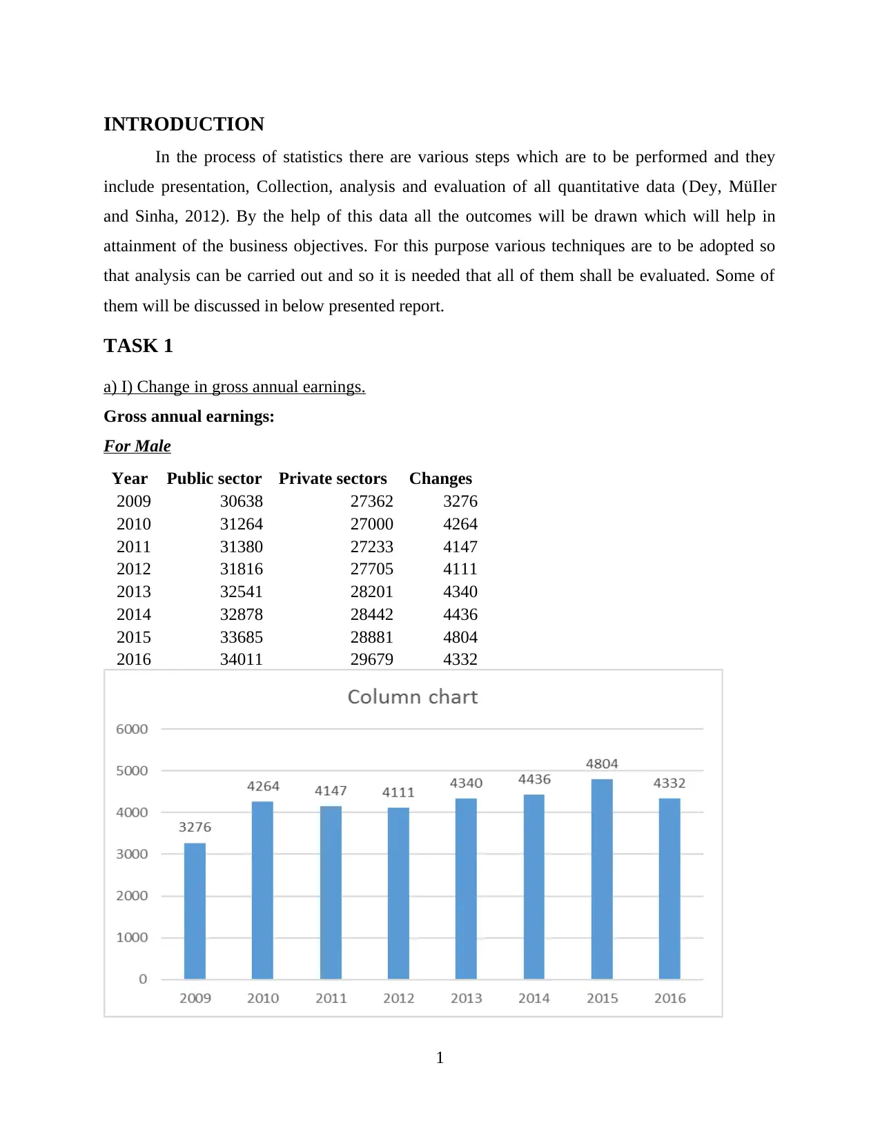
For Male
Year Public sector Private sectors Changes
2009 30638 27362 3276
2010 31264 27000 4264
2011 31380 27233 4147
2012 31816 27705 4111
2013 32541 28201 4340
2014 32878 28442 4436
2015 33685 28881 4804
2016 34011 29679 4332
1

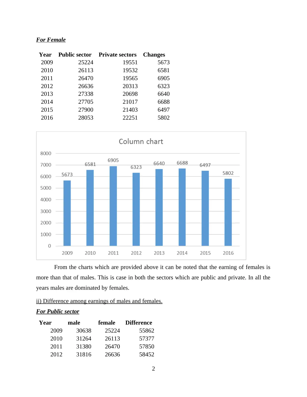
For Female
Year Public sector Private sectors Changes
2009 25224 19551 5673
2010 26113 19532 6581
2011 26470 19565 6905
2012 26636 20313 6323
2013 27338 20698 6640
2014 27705 21017 6688
2015 27900 21403 6497
2016 28053 22251 5802
From the charts which are provided above it can be noted that the earning of females is
more than that of males. This is case in both the sectors which are public and private. In all the
years males are dominated by females.
ii) Difference among earnings of males and females.
For Public sector
Year male female Difference
2009 30638 25224 55862
2010 31264 26113 57377
2011 31380 26470 57850
2012 31816 26636 58452
2

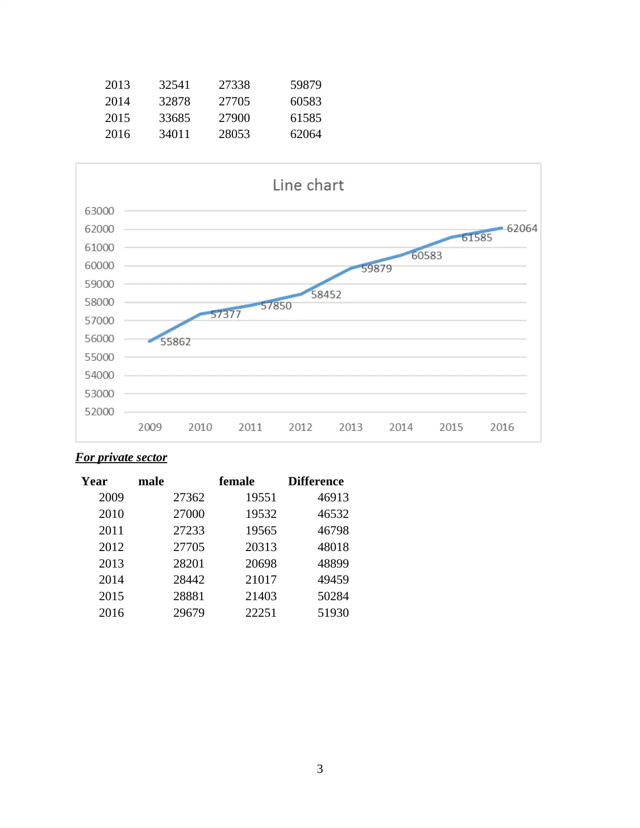
2013 32541 27338 59879
2014 32878 27705 60583
2015 33685 27900 61585
2016 34011 28053 62064
For private sector
Year male female Difference
2009 27362 19551 46913
2010 27000 19532 46532
2011 27233 19565 46798
2012 27705 20313 48018
2013 28201 20698 48899
2014 28442 21017 49459
2015 28881 21403 50284
2016 29679 22251 51930
3

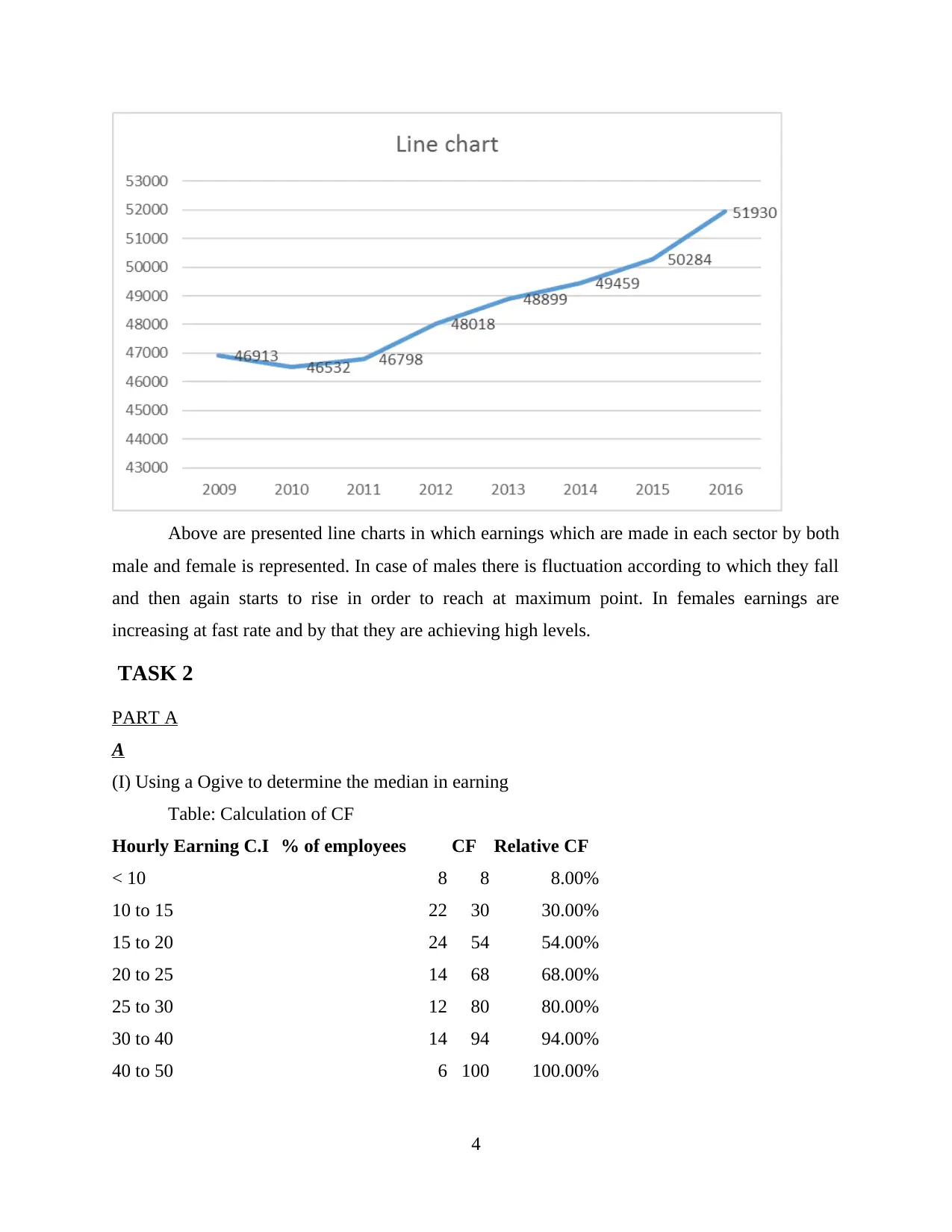
Above are presented line charts in which earnings which are made in each sector by both
male and female is represented. In case of males there is fluctuation according to which they fall
and then again starts to rise in order to reach at maximum point. In females earnings are
increasing at fast rate and by that they are achieving high levels.
TASK 2
PART A
A
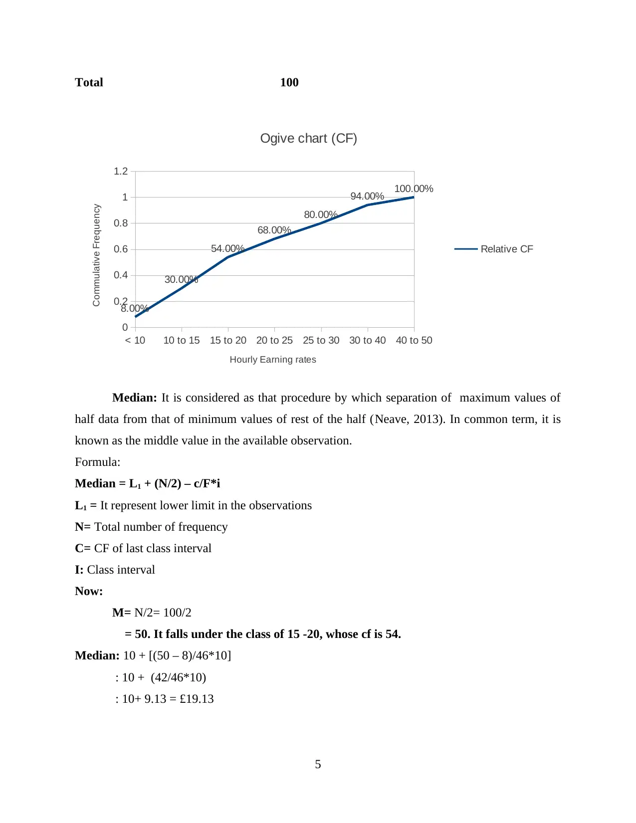
(I) Using a Ogive to determine the median in earning
Table: Calculation of CF
Hourly Earning C.I % of employees CF Relative CF
< 10 8 8 8.00%
10 to 15 22 30 30.00%
15 to 20 24 54 54.00%
20 to 25 14 68 68.00%
25 to 30 12 80 80.00%
30 to 40 14 94 94.00%
40 to 50 6 100 100.00%
4

Total 100
< 10 10 to 15 15 to 20 20 to 25 25 to 30 30 to 40 40 to 50
0
0.2
0.4
0.6
0.8
1
1.2
8.00%
30.00%
54.00%
68.00%
80.00%
94.00% 100.00%
Ogive chart (CF)
Relative CF
Hourly Earning rates
Commulative Frequency
Median: It is considered as that procedure by which separation of maximum values of
half data from that of minimum values of rest of the half (Neave, 2013). In common term, it is
known as the middle value in the available observation.
Formula:
Median = L1 + (N/2) – c/F*i
L1 = It represent lower limit in the observations
N= Total number of frequency
C= CF of last class interval
I: Class interval
Now:
M= N/2= 100/2
= 50. It falls under the class of 15 -20, whose cf is 54.
Median: 10 + [(50 – 8)/46*10]
: 10 + (42/46*10)
: 10+ 9.13 = £19.13
5

Quartile: The of the data are categories into various set mostly in three. Each of them is
equal to those segment which is categories into four specific tasks. The middle number among
the smallest data series and median values of data is called as Q1 (Haimes, 2015). Other are
divided into Q2 and Q3 between highest and middle values of the data series in the given
observations.
Quartile calculation:
Q1: N/4
: 100 /4 = 25. It is falls under the group of 10 -15 with the CF of 30.
Q1= 10 + (25- 8)/22*10
= 10+ 17 /22 *10
= 10+7.7 = £17.7
Q3 = 3(N+1)/4 = 3(110/4)= 75.7
It will fall under the class interval of 25 -30 with the CF of 80
Q3= 25 + (75 – 68)/12 *10
= 25 + (7/12*10)
= 25+ 5.8 = £ 30.8
From the above calculation, it has been found that Hourly earning is been computed by
using median and quartile values. In which is was seen that £19.13 which is more near to wages
rate of £19.13 per hours. It represent that 50% of the total people are base yield hourly wages
paid are under £19. According to quartile values, 25% of the workers are getting a minimum
wages rate or equal to £17.7 which is more closer to 18 per hours. While, 75% of them has paid
at £30 per hours. After summarising all the results, it has been concluded that only 6 people are
getting minimum of the wages which belong to the category of 40-50.
II): Computation of mean and standard deviation
Hourly Earning Frequency
Mid
value F * X
<10 8 5 40
10 but under 15 22 12.5 275
15 to 20 24 17.5 420
20 to 25 14 22.5 315
25 to 30 12 27.5 330
6

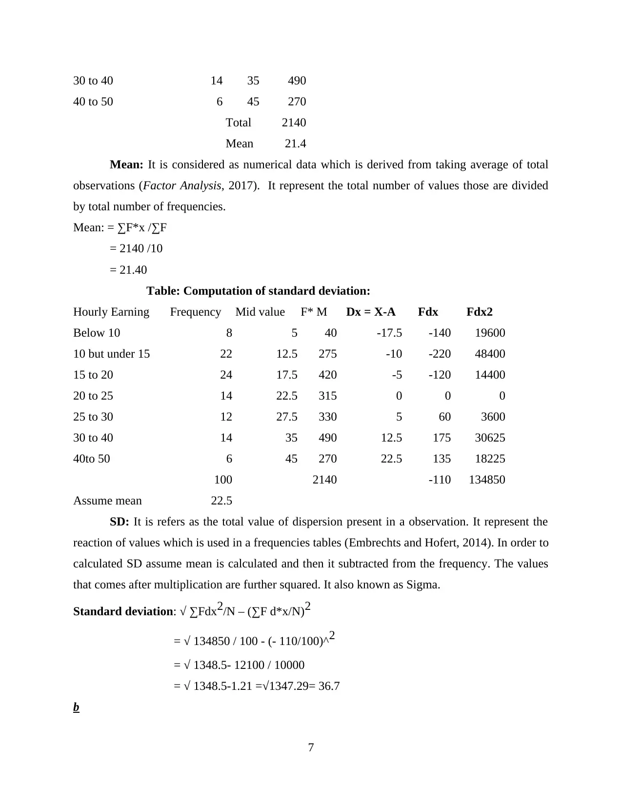
30 to 40 14 35 490
40 to 50 6 45 270
Total 2140
Mean 21.4
Mean: It is considered as numerical data which is derived from taking average of total
observations (Factor Analysis, 2017). It represent the total number of values those are divided
by total number of frequencies.
Mean: = ∑F*x /∑F
= 2140 /10
= 21.40
Table: Computation of standard deviation:
Hourly Earning Frequency Mid value F* M Dx = X-A Fdx Fdx2
Below 10 8 5 40 -17.5 -140 19600
10 but under 15 22 12.5 275 -10 -220 48400
15 to 20 24 17.5 420 -5 -120 14400
20 to 25 14 22.5 315 0 0 0
25 to 30 12 27.5 330 5 60 3600
30 to 40 14 35 490 12.5 175 30625
40to 50 6 45 270 22.5 135 18225
100 2140 -110 134850
Assume mean 22.5
SD: It is refers as the total value of dispersion present in a observation. It represent the
reaction of values which is used in a frequencies tables (Embrechts and Hofert, 2014). In order to
calculated SD assume mean is calculated and then it subtracted from the frequency. The values
that comes after multiplication are further squared. It also known as Sigma.
Standard deviation: √ ∑Fdx2/N – (∑F d*x/N)2
= √ 134850 / 100 - (- 110/100)^2
= √ 1348.5- 12100 / 10000
= √ 1348.5-1.21 =√1347.29= 36.7
b
7

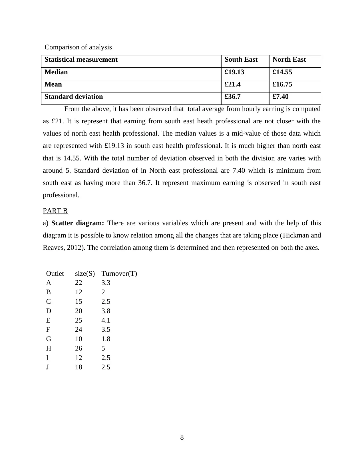
Comparison of analysis
Statistical measurement South East North East
Median £19.13 £14.55
Mean £21.4 £16.75
Standard deviation £36.7 £7.40
From the above, it has been observed that total average from hourly earning is computed
as £21. It is represent that earning from south east heath professional are not closer with the
values of north east health professional. The median values is a mid-value of those data which
are represented with £19.13 in south east health professional. It is much higher than north east
that is 14.55. With the total number of deviation observed in both the division are varies with
around 5. Standard deviation of in North east professional are 7.40 which is minimum from
south east as having more than 36.7. It represent maximum earning is observed in south east
professional.
PART B
a) Scatter diagram: There are various variables which are present and with the help of this
diagram it is possible to know relation among all the changes that are taking place (Hickman and
Reaves, 2012). The correlation among them is determined and then represented on both the axes.
Outlet size(S) Turnover(T)
A 22 3.3
B 12 2
C 15 2.5
D 20 3.8
E 25 4.1
F 24 3.5
G 10 1.8
H 26 5
I 12 2.5
J 18 2.5
8

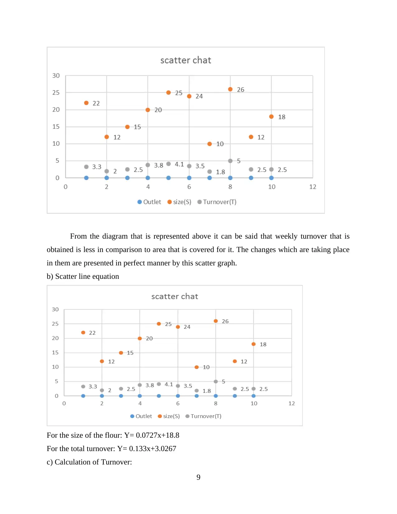
From the diagram that is represented above it can be said that weekly turnover that is
obtained is less in comparison to area that is covered for it. The changes which are taking place
in them are presented in perfect manner by this scatter graph.
b) Scatter line equation
For the size of the flour: Y= 0.0727x+18.8
For the total turnover: Y= 0.133x+3.0267
c) Calculation of Turnover:
9

Y= 0.133x + 3.0267
= 0.133 * 30 + 3.0267
= 3.99 + 3.0267 = 7.0167 per Sq m
d) Correlation Coefficient calculation
Outlet size(S)
Turnover
(T)
A 22 3.3
B 12 2
C 15 2.5
D 20 3.8
E 25 4.1
F 24 3.5
G 10 1.8
H 26 5
I 12 2.5
J 18 2.5
Coefficient
correlation 0.91
Range
Minimum 1.8
Maximum 5
e) For the purpose of knowing the relation in between cause and effect, all the data shall be
represented and that is considered under statistical validity (Heizer, 2016). By this it is
determined that is there any relation which exist and how it will be affected if any change is
occurred. There may be error which is present or can be due to the measurement mistakes. The
main factors that shall be considered under this are as follows:
 Selection effect: This is the factor by which turnover will be affected. It is identified that
by the help of the selection that is made. Is it possible to get such results which are best
for all. Proper method and techniques are to be used so that effect can be determined.
 Testing effect: When all the values are to be identified from the available data then this
is used. This is carried out so that accurate results can be ascertained.
TASK 3
Use of statistical methods for planning.
10

In order to get more positive and reliable outcomes all of these methods shall be used. By
the use of all information it is possible to know the accurate outcomes. By using statistical
methods, numerical data can be determined (Linoff and Berry, 2011). It is difficult to handle
statistics when there is incline data. The methods that are used for this purpose are standard
deviation and mean. In addition to them F test, regression and t test can also be taken into
consideration. Some of the methods that can be used are as follows:
Chi-square test: This is the test under which chi squared distribution is used for sampling
distribution and this is done in case of Null hypothesis.
Analysis of variance: By the help of this the variable which are present are compared. Here the
difference that exist among means of various variables are analysed.
Correlation: There is some or other mutual relation that is present among any two variables and
it can be represented with the help of this tool (McNeil, Frey and Embrechts, 2015). By this
comparison can be made and it can be identified that in which will the high relation exist.
Factor analysis: There are various low numbers which are considered as factors and by this
technique variability is determined between the variables that are correlated.
a) Total deliveries in year
Total working days = 365-5 = 360
Time taken by one delivery: 12 days
Total deliveries = 360/12 = 30 deliveries
b) Number of bottles in each delivery
Total bottles demand = 450000
Total deliveries = 30
Units per delivery = 450000/30 = 15000 bottles
c) Economic order quantity
This is the quantity at which company will be gaining best advantage.
EOQ=√2RO/C
=√2*450000*20/0.50
=6000 bottles
11

d) Variations and recommendation
In production there are various variable cost and together they make total cost of product.
In this material, labour and all other expenses are considered (Venables and Ripley, 2013).
Variable expenses change with change in production on direct basis. So for this it is required that
relationship among them shall be understood by management. The stock is to be maintained at
EOQ level as that is best for company. For the achievement of best results it is needed that
proper strategies shall be formulated.
TASK 4
a) Findings communication by using line chart
a) Gross annual earnings
For Male
Year Public sector Private sectors Changes
2009 30638 27362 3276
2010 31264 27000 4264
2011 31380 27233 4147
2012 31816 27705 4111
2013 32541 28201 4340
2014 32878 28442 4436
2015 33685 28881 4804
2016 34011 29679 4332
12

Gross Annual earnings
For Female
Year Public sector Private sectors Changes
2009 25224 19551 5673
2010 26113 19532 6581
2011 26470 19565 6905
2012 26636 20313 6323
2013 27338 20698 6640
2014 27705 21017 6688
2015 27900 21403 6497
2016 28053 22251 5802
13

By the help of the charts that are presented above gross earnings of males and females are
analyzed. The line is fluctuating in both the cases as in females it increases then declines and
after that again starts to rise at constant pace. In ales also this pattern is followed but the earnings
are more for females then males.
b) Representation through ogives.
Hourly Earning % of employees CF
Below 10 8 8
10 but under 15 22 30
15 to 20 24 54
20 to 25 14 68
25 to 30 12 80
30 to 40 14 94
40 to 50 6 100
14

By the help of this ogive chart the earnings of employees in organisation is represented
for an hour. It can be seen that the starting point for cumulative frequency is 8 which reaches till
54. thereafter a fall can be noted after which constant increase is made. So for improvement it is
recommended that earnings shall be increased for those falling under 20 to 25 range and decrease
shall be done for below 10 category.
CONCLUSION
From the above report it can be concluded that for the analysation of all the data it si
required that statistical management shall be adopted as it is most effective. Also all the central
tendency measures are used for drawing conclusions. On the basis of that business can be
improved.
15