Normality of Variables in Hypothesis Testing

The provided assignment content discusses the normality probability plots and hypothesis testing of various independent variables, including NP/TA, TL/TA, WC/TA, QE/TL, PS/TS, TC/TS, and OE/TL. The results show that some variables have a linear normal trend while others follow a normal trend. Hypothesis tests were conducted using the two-independent-sample t-test with unequal variances to determine if there are statistically significant differences between certain groups. Some findings suggest no statistically significant difference, while others indicate a statistically significant difference.

Statistics For Management Decision
Assessment -2
Student Id
[Pick the date]

Question 1
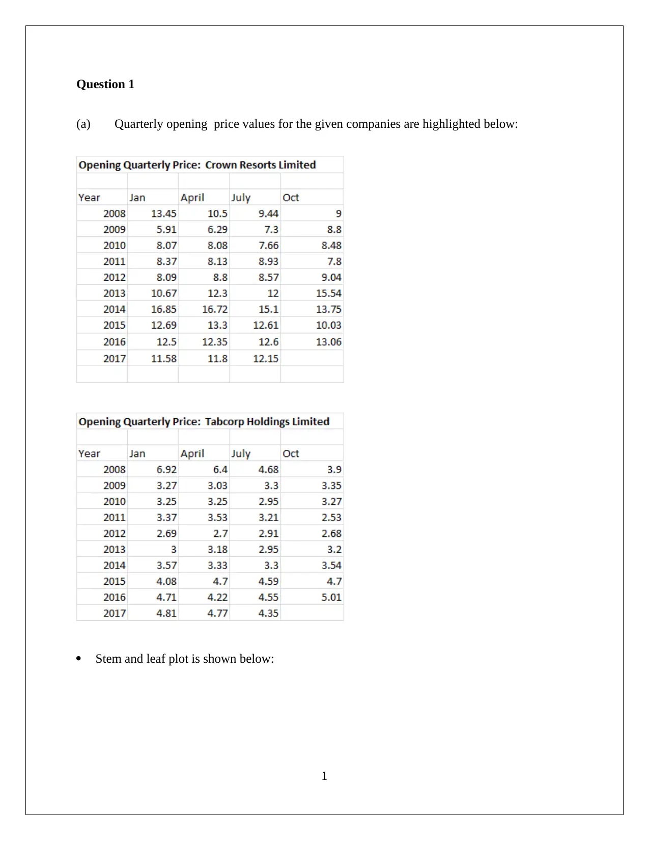
(a) Quarterly opening price values for the given companies are highlighted below:
 Stem and leaf plot is shown below:
1

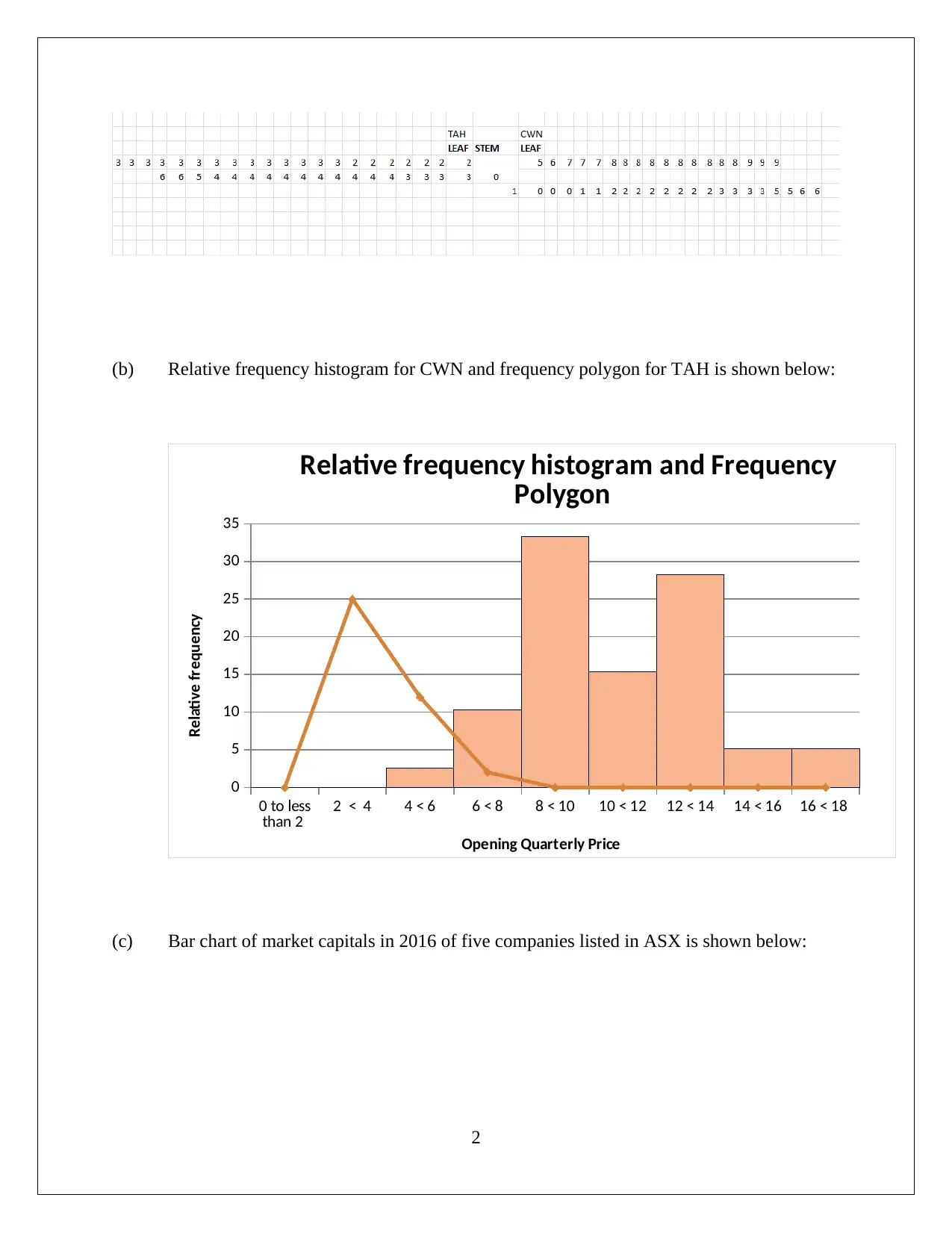
(b) Relative frequency histogram for CWN and frequency polygon for TAH is shown below:
0 to less
than 2 2 < 4 4 < 6 6 < 8 8 < 10 10 < 12 12 < 14 14 < 16 16 < 18
0
5
10
15
20
25
30
35
Relative frequency histogram and Frequency
Polygon
Opening Quarterly Price
Relative frequency
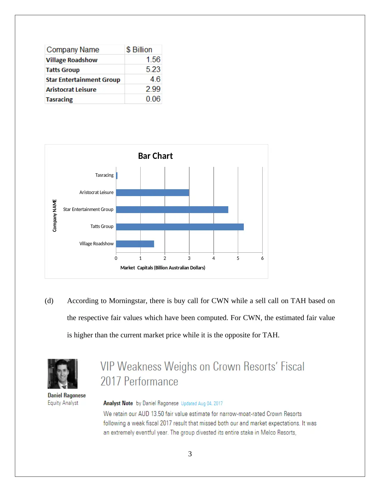
(c) Bar chart of market capitals in 2016 of five companies listed in ASX is shown below:
2

Village Roadshow
Tatts Group
Star Entertainment Group
Aristocrat Leisure
Tasracing
0 1 2 3 4 5 6
Bar Chart
Market Capitals (Billion Australian Dollars)
Company NAME
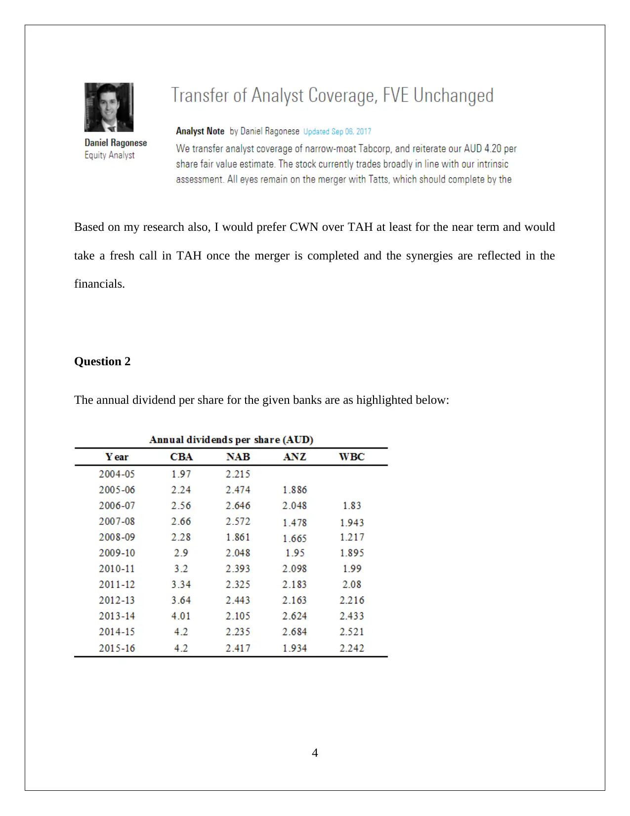
(d) According to Morningstar, there is buy call for CWN while a sell call on TAH based on
the respective fair values which have been computed. For CWN, the estimated fair value
is higher than the current market price while it is the opposite for TAH.
3

Based on my research also, I would prefer CWN over TAH at least for the near term and would
take a fresh call in TAH once the merger is completed and the synergies are reflected in the
financials.
Question 2
The annual dividend per share for the given banks are as highlighted below:
4

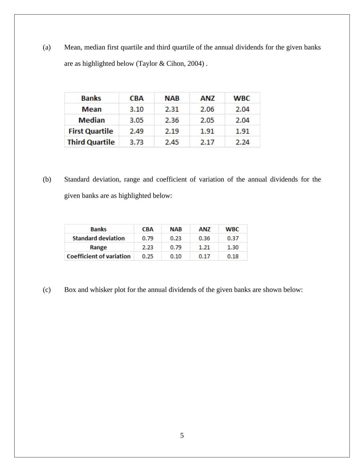
(a) Mean, median first quartile and third quartile of the annual dividends for the given banks
are as highlighted below (Taylor & Cihon, 2004) .
(b) Standard deviation, range and coefficient of variation of the annual dividends for the
given banks are as highlighted below:
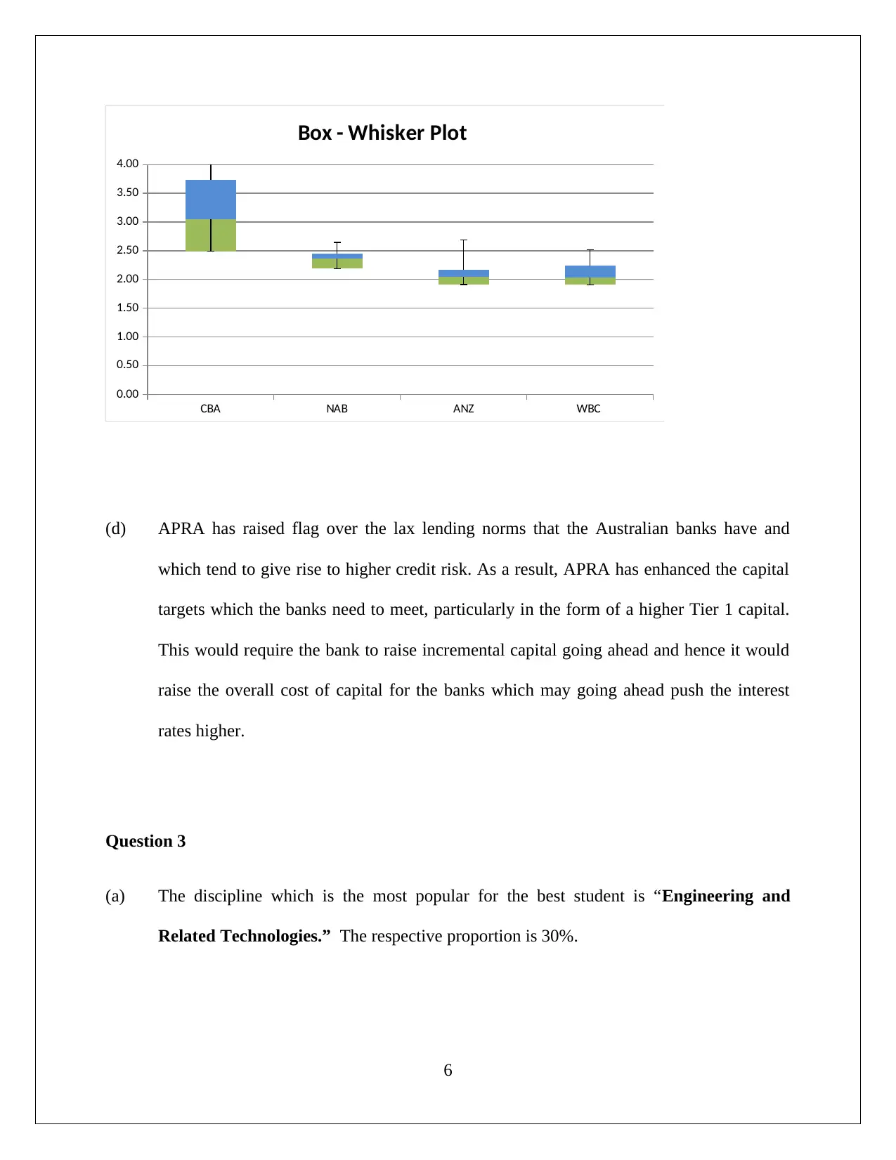
(c) Box and whisker plot for the annual dividends of the given banks are shown below:
5

CBA NAB ANZ WBC
0.00
0.50
1.00
1.50
2.00
2.50
3.00
3.50
4.00
Box - Whisker Plot
(d) APRA has raised flag over the lax lending norms that the Australian banks have and
which tend to give rise to higher credit risk. As a result, APRA has enhanced the capital
targets which the banks need to meet, particularly in the form of a higher Tier 1 capital.
This would require the bank to raise incremental capital going ahead and hence it would
raise the overall cost of capital for the banks which may going ahead push the interest
rates higher.
Question 3
(a) The discipline which is the most popular for the best student is “Engineering and
Related Technologies.” The respective proportion is 30%.
6

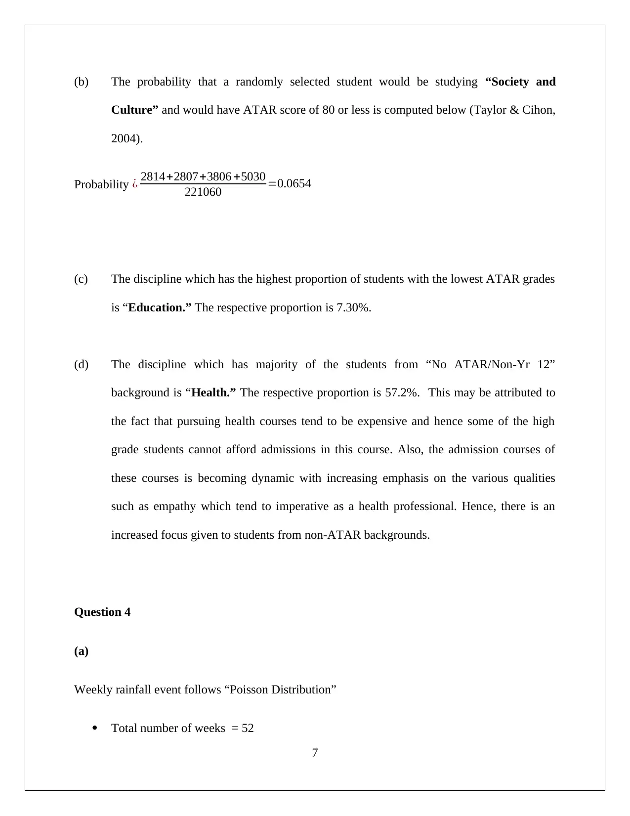
(b) The probability that a randomly selected student would be studying “Society and
Culture” and would have ATAR score of 80 or less is computed below (Taylor & Cihon,
2004).
Probability ¿ 2814+2807+3806 +5030
221060 =0.0654
(c) The discipline which has the highest proportion of students with the lowest ATAR grades
is “Education.” The respective proportion is 7.30%.
(d) The discipline which has majority of the students from “No ATAR/Non-Yr 12”
background is “Health.” The respective proportion is 57.2%. This may be attributed to
the fact that pursuing health courses tend to be expensive and hence some of the high
grade students cannot afford admissions in this course. Also, the admission courses of
these courses is becoming dynamic with increasing emphasis on the various qualities
such as empathy which tend to imperative as a health professional. Hence, there is an
increased focus given to students from non-ATAR backgrounds.
Question 4
(a)
Weekly rainfall event follows “Poisson Distribution”
 Total number of weeks = 52
7

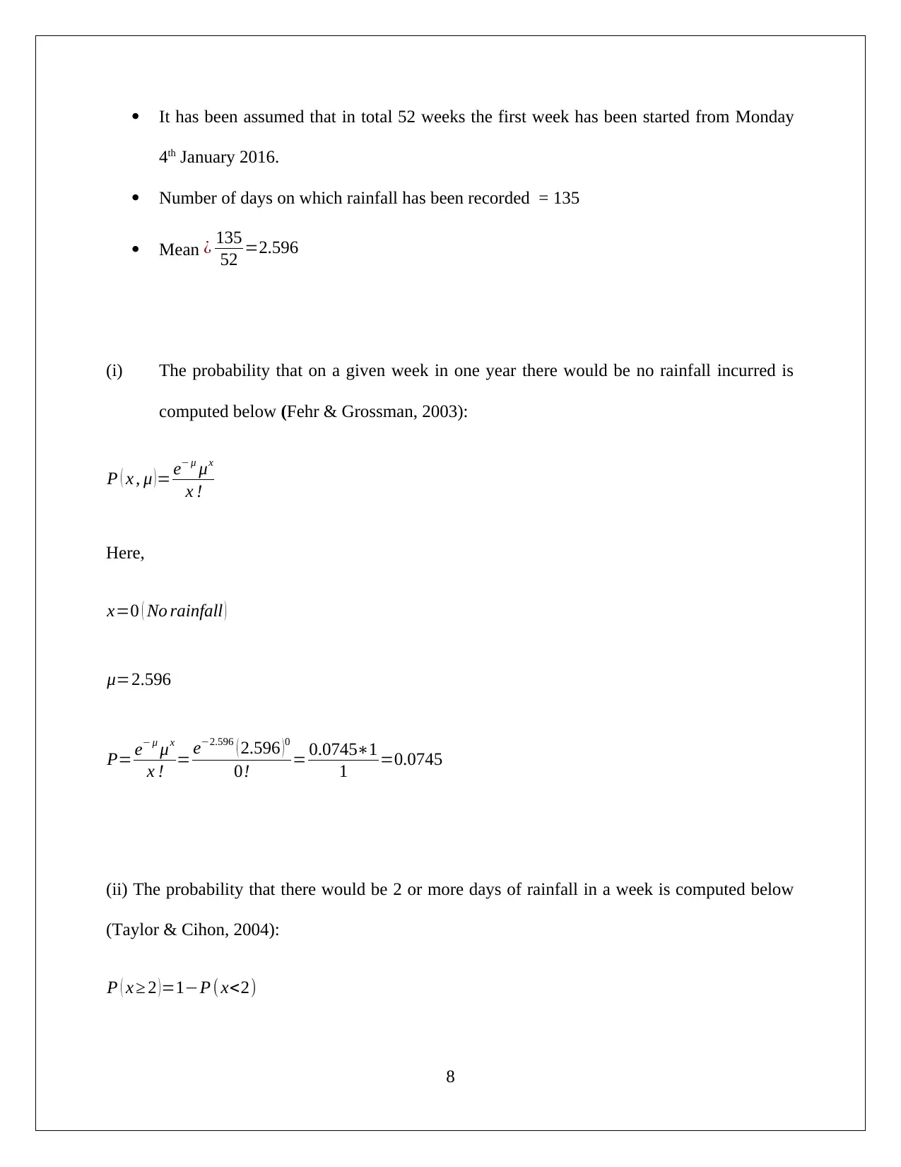
 It has been assumed that in total 52 weeks the first week has been started from Monday
4th January 2016.
 Number of days on which rainfall has been recorded = 135
 Mean ¿ 135
52 =2.596
(i) The probability that on a given week in one year there would be no rainfall incurred is
computed below (Fehr & Grossman, 2003):
P ( x , μ )= e− μ μx
x !
Here,
x=0 ( No rainfall )
μ=2.596
P= e− μ μx
x ! = e−2.596 ( 2.596 )0
0! = 0.0745∗1
1 =0.0745
(ii) The probability that there would be 2 or more days of rainfall in a week is computed below
(Taylor & Cihon, 2004):
P ( x ≥ 2 )=1−P ( x<2)
8

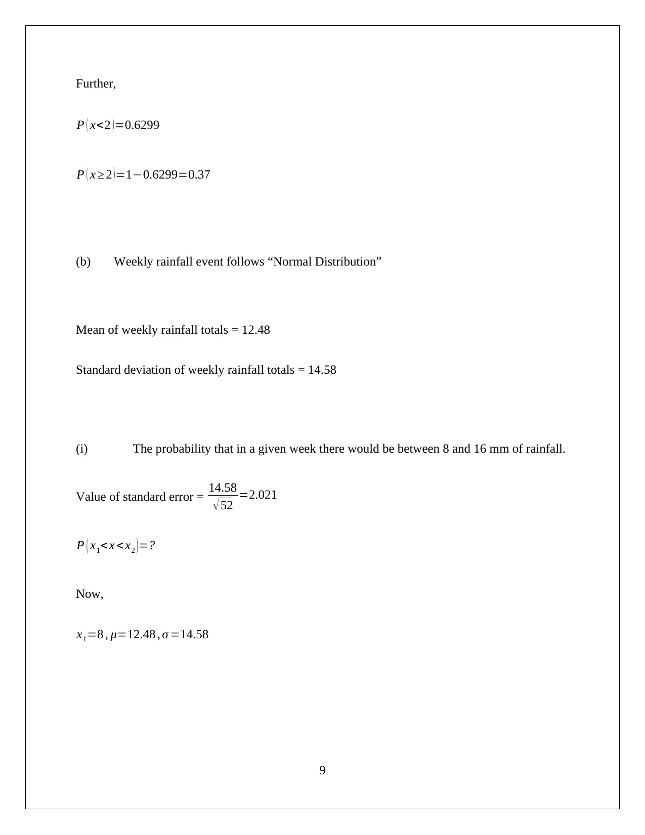
Further,
P ( x<2 )=0.6299
P ( x ≥ 2 ) =1−0.6299=0.37
(b) Weekly rainfall event follows “Normal Distribution”
Mean of weekly rainfall totals = 12.48
Standard deviation of weekly rainfall totals = 14.58
(i) The probability that in a given week there would be between 8 and 16 mm of rainfall.
Value of standard error = 14.58
√52 =2.021
P ( x1<x < x2 )=?
Now,
x1=8 , μ=12.48 , σ =14.58
9

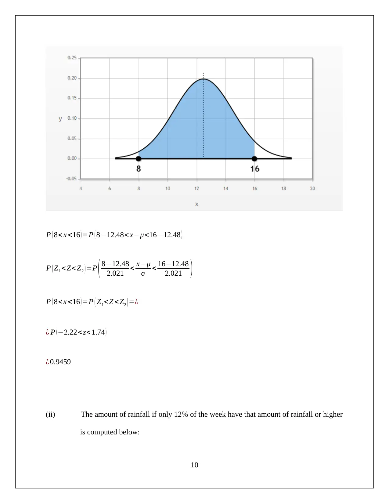
P ( 8< x <16 )=P ( 8−12.48< x−μ<16−12.48 )
P ( Z1 < Z< Z2 )=P ( 8−12.48
2.021 < x−μ
σ < 16−12.48
2.021 )
P ( 8< x <16 ) =P ( Z1< Z <Z2 ) =¿
¿ P ( −2.22< z< 1.74 )
¿ 0.9459
(ii) The amount of rainfall if only 12% of the week have that amount of rainfall or higher
is computed below:
10

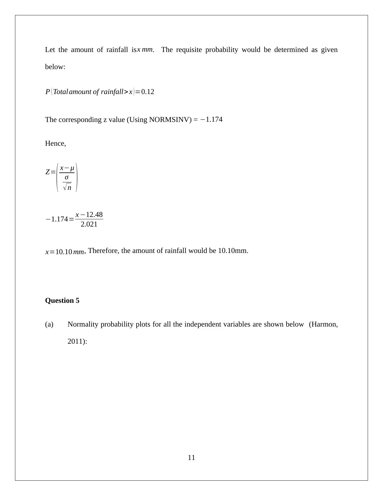
Let the amount of rainfall isx mm. The requisite probability would be determined as given
below:
P ( Totalamount of rainfall>x )=0.12
The corresponding z value (Using NORMSINV) = −1.174
Hence,
Z=
( x−μ
σ
√ n )
−1.174= x −12.48
2.021
x=10.10 mm, Therefore, the amount of rainfall would be 10.10mm.
Question 5
(a) Normality probability plots for all the independent variables are shown below (Harmon,
2011):
11

-500 -400 -300 -200 -100 0 100
-4
-3
-2
-1
0
1
2
3
4
Normal Probability Plot : NP/TA
Data
Quantiles
It can be seen from the above Normal Probability Plot that the parameters of variable NP/TA is
showing linear normal trend.
0 10 20 30 40 50 60 70 80
-4
-3
-2
-1
0
1
2
3
4
Normality Probability Plot : TL/TA
Data
Quantiles
It can be seen from the above Normal Probability Plot that the parameters of TL/TA is showing
normal trend.
12

-80 -70 -60 -50 -40 -30 -20 -10 0 10
-4
-3
-2
-1
0
1
2
3
4
Normal Probability Plot : WC/ TA
Data
Quantiles
It can be seen from the above highlighted Normal Probability Plot that the parameters of WC/TA
is showing normal trend.
-100 0 100 200 300 400 500 600 700 800
-4
-3
-2
-1
0
1
2
3
4
Normal Probability Plot: QE /TL
Data
Quantiles
It can be seen from the above Normal Probability Plot that the parameters of QE/TL variable is
showing linear normal trend.
13

-16 -14 -12 -10 -8 -6 -4 -2 0 2
-4
-3
-2
-1
0
1
2
3
4
Normal Probability Plot : PS/TS
Data
Quantiles
It can be seen from the above Normal Probability Plot that the parameters of the variable PS/TS
is showing linear normal trend.
-5 0 5 10 15 20 25
-4
-3
-2
-1
0
1
2
3
4
Normal Probability Plot : TC/TS
Data
Quantiles
14

It is apparent from the above Normal Probability Plot that the parameters of TC/TS is showing
linear normal trend.
(b) Confidence interval for all the independent variables is determined based on the given
formula (Fehr & Grossman, 2003).
Lower limit of 95 % confidence interval=Mean−Confidence level
Upper limit of 95 % confidence interval=Mean+Confidence level
15

(c) Hypothesis testing
(1) NP/TA
The relevant hypotheses are indicated below.
16

Null Hypothesis: μBankruptcy=0 = μBankruptcy=1
Alternative Hypothesis: μBankruptcy=0 ≠ μBankruptcy=1
The appropriate test to be deployed in a two independent sample t test with unequal variances
whose excel output has been indicated below.
Relevant p value = 0.2065
Decision: Failure to reject null hypothesis since p value is greater than significance level
Conclusion: No statistically significant difference
(2) PS TS
The relevant hypotheses are indicated below.
Null Hypothesis: μBankruptcy=0 = μBankruptcy=1
Alternative Hypothesis: μBankruptcy=0 ≠ μBankruptcy=1
17

The appropriate test to be deployed in a two independent sample t test with unequal variances
whose excel output has been indicated below (Koch, 2013).
Relevant p value = 0.00
Decision: Reject null hypothesis since p value is lower than significance level
Conclusion: Statistically significant difference (Lehman & Romano, 2006).
(3) TC TS
The relevant hypotheses are indicated below.
Null Hypothesis: μBankruptcy=0 = μBankruptcy=1
Alternative Hypothesis: μBankruptcy=0 ≠ μBankruptcy=1
The appropriate test to be deployed in a two independent sample t test with unequal variances
whose excel output has been indicated below.
18

Relevant p value = 0.00
Decision: Reject null hypothesis since p value is lower than significance level
Conclusion: Statistically significant difference
(4) TL TA
The relevant hypotheses are indicated below.
Null Hypothesis: μBankruptcy=0 = μBankruptcy=1
Alternative Hypothesis: μBankruptcy=0 ≠ μBankruptcy=1
The appropriate test to be deployed in a two independent sample t test with unequal variances
whose excel output has been indicated below.
19

Relevant p value = 0.0005
Decision: Reject null hypothesis since p value is lower than significance level
Conclusion: Statistically significant difference
(5) WC TA
The relevant hypotheses are indicated below.
Null Hypothesis: μBankruptcy=0 = μBankruptcy=1
Alternative Hypothesis: μBankruptcy=0 ≠ μBankruptcy=1
The appropriate test to be deployed in a two independent sample t test with unequal variances
whose excel output has been indicated below (Lehman & Romano, 2006).
20

Relevant p value = 0.0007
Decision: Reject null hypothesis since p value is lower than significance level
Conclusion: Statistically significant difference
(6) OE TL
The relevant hypotheses are indicated below.
Null Hypothesis: μBankruptcy=0 = μBankruptcy=1
Alternative Hypothesis: μBankruptcy=0 ≠ μBankruptcy=1
The appropriate test to be deployed in a two independent sample t test with unequal variances
whose excel output has been indicated below (Lehman & Romano, 2006).
21

Relevant p value = 0.1248
Decision: Failure to reject null hypothesis since p value is greater than significance level
Conclusion: No statistically significant difference (Taylor & Cihon, 2004).
22