EOQ Model and Healthcare Professionals Earnings

The assignment delves into the relationship between Economic Order Quantity (EOQ) models and healthcare professional earnings. It utilizes statistical analysis, including mean, median, and standard deviation, to compare earning capacities in different healthcare regions (Southeast and Northeast). The analysis aims to demonstrate how EOQ measurement can be adapted for cost control and capacity analysis in non-traditional business contexts like healthcare. The assignment includes visual representations of the data using ogive charts and tables.

STATISTICS FOR
MANAGEMENT

TABLE OF CONTENTS
INTRODUCTION...........................................................................................................................1
TASK 1............................................................................................................................................1
(a) 1 Measuring the Net Annual income for private and public sector and relevant changes1
(a) 2 Differences as well as gap between earning capacity of male and female annual revenue2
TASK 2............................................................................................................................................4
(A) Analysing the Hour basis Paying rates of Health professionals in South East................4
1 Estimating the Hourly basis Median with Ogive chart.......................................................4
2 Measuring the Standard deviation and Mean on the basis of Hourly Earnings..................5
(B) Analysing the North East Health professionals as compared to South East....................7
1. Analysing the Scatter Diagram as well as Discussion between Average turnover and Floor
area.........................................................................................................................................7
2. Interpretation of Equation of Line of best fit......................................................................8
3. Measuring the turnover on the basis of equation................................................................8
4. Measurement of regression and the correlation coefficient...............................................9
5. Analysing the Statistical Validity as well as factors affecting Average weekly turnover..9
TASK 3..........................................................................................................................................10
(B) Measuring the supply of olive oil bottles.......................................................................10
1. Calculating the numbers of delivery made in each year...................................................10
2. Analysing the numbers of selling for olive oil in each Supply........................................10
3. Evaluating the calculations for EOQ with the help of statistical measurement...............10
4. Recommendation based on the Variable cost model and EOQ measurement.................10
TASK 4..........................................................................................................................................11
1. Findings based on the data set in the task 2......................................................................11
2 Demonstrating the diagram on the basis of task 1.............................................................12
3 Presenting the diagram on the basis of data used in Task 2 in table 2..............................12
CONCLUSION..............................................................................................................................12
REFERENCES..............................................................................................................................14

INTRODUCTION
Statistics management is the technique where the entity can be able analyse the financial
position of the organisation on behalf of various data set. In the present there will be calculations
based on collecting the data, measuring the statistics of that as well as interpreting such analysis.
Hence, there will be comparison over the performance of the individual and the companies as per
their operating years. Thus, these research will be helpful for the firm in as well as for the
professionals in making the favourable solutions and effective planning for future tasks.
However, there will be calculation of regression, correlation, standard deviation, mean and
median which will facilitate the favourable results or outcomes. Thus, there will be calculation
based on the EOQ measurements which will be beneficial for the professionals to analyse the
cost incurred per order.
TASK 1
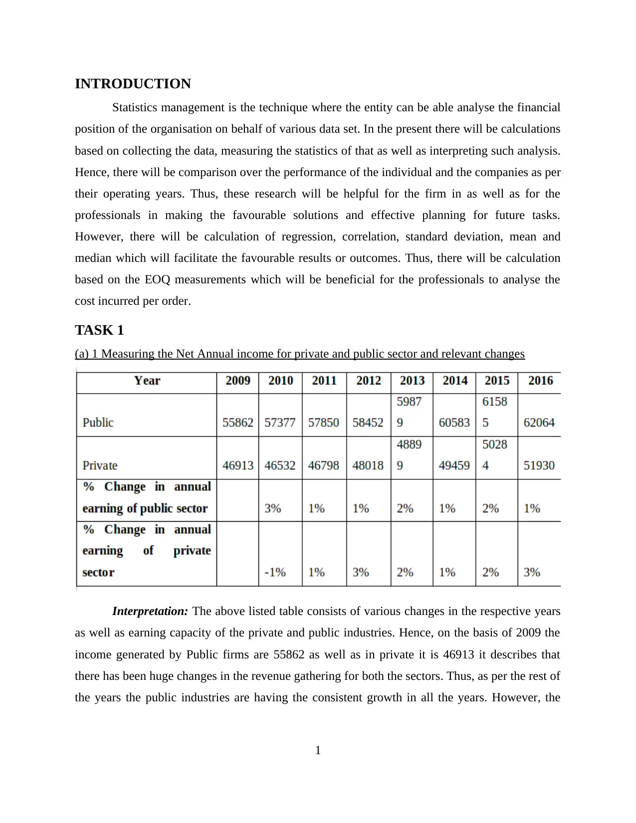
(a) 1 Measuring the Net Annual income for private and public sector and relevant changes
Interpretation: The above listed table consists of various changes in the respective years
as well as earning capacity of the private and public industries. Hence, on the basis of 2009 the
income generated by Public firms are 55862 as well as in private it is 46913 it describes that
there has been huge changes in the revenue gathering for both the sectors. Thus, as per the rest of
the years the public industries are having the consistent growth in all the years. However, the
1

private sector do not have the favourable growth in all such years as compared with the public
sector (Schmerler and et.al., 2016).
(a) 2 Differences as well as gap between earning capacity of male and female annual revenue
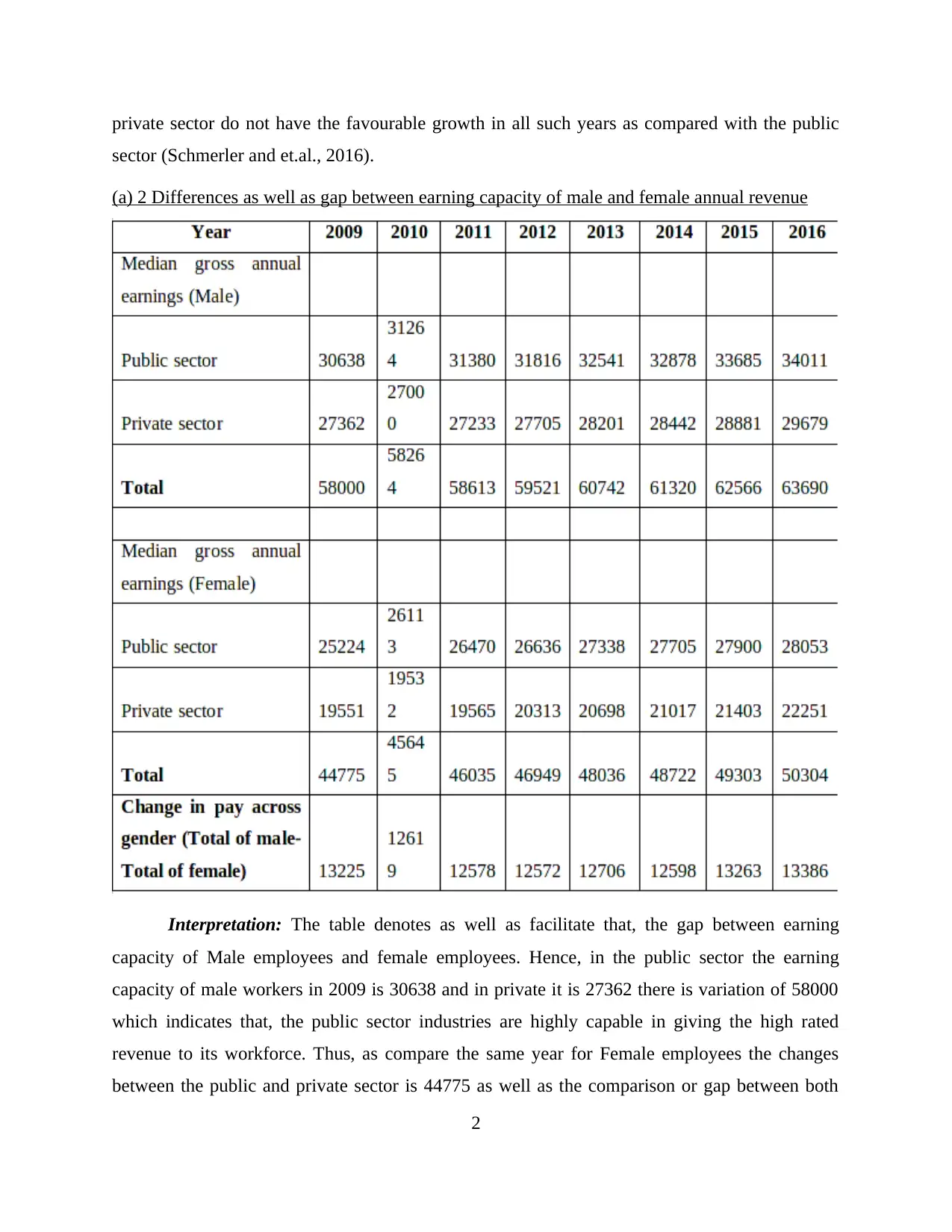
Interpretation: The table denotes as well as facilitate that, the gap between earning
capacity of Male employees and female employees. Hence, in the public sector the earning
capacity of male workers in 2009 is 30638 and in private it is 27362 there is variation of 58000
which indicates that, the public sector industries are highly capable in giving the high rated
revenue to its workforce. Thus, as compare the same year for Female employees the changes
between the public and private sector is 44775 as well as the comparison or gap between both
2

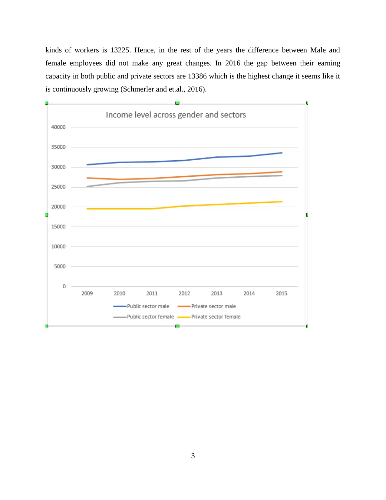
kinds of workers is 13225. Hence, in the rest of the years the difference between Male and
female employees did not make any great changes. In 2016 the gap between their earning
capacity in both public and private sectors are 13386 which is the highest change it seems like it
is continuously growing (Schmerler and et.al., 2016).
3

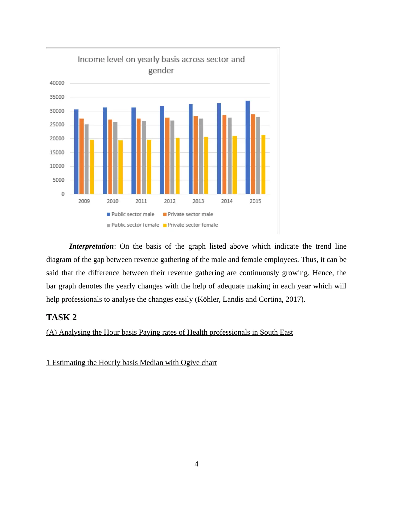
Interpretation: On the basis of the graph listed above which indicate the trend line
diagram of the gap between revenue gathering of the male and female employees. Thus, it can be
said that the difference between their revenue gathering are continuously growing. Hence, the
bar graph denotes the yearly changes with the help of adequate making in each year which will
help professionals to analyse the changes easily (Köhler, Landis and Cortina, 2017).
TASK 2
(A) Analysing the Hour basis Paying rates of Health professionals in South East
1 Estimating the Hourly basis Median with Ogive chart
4

Illustration
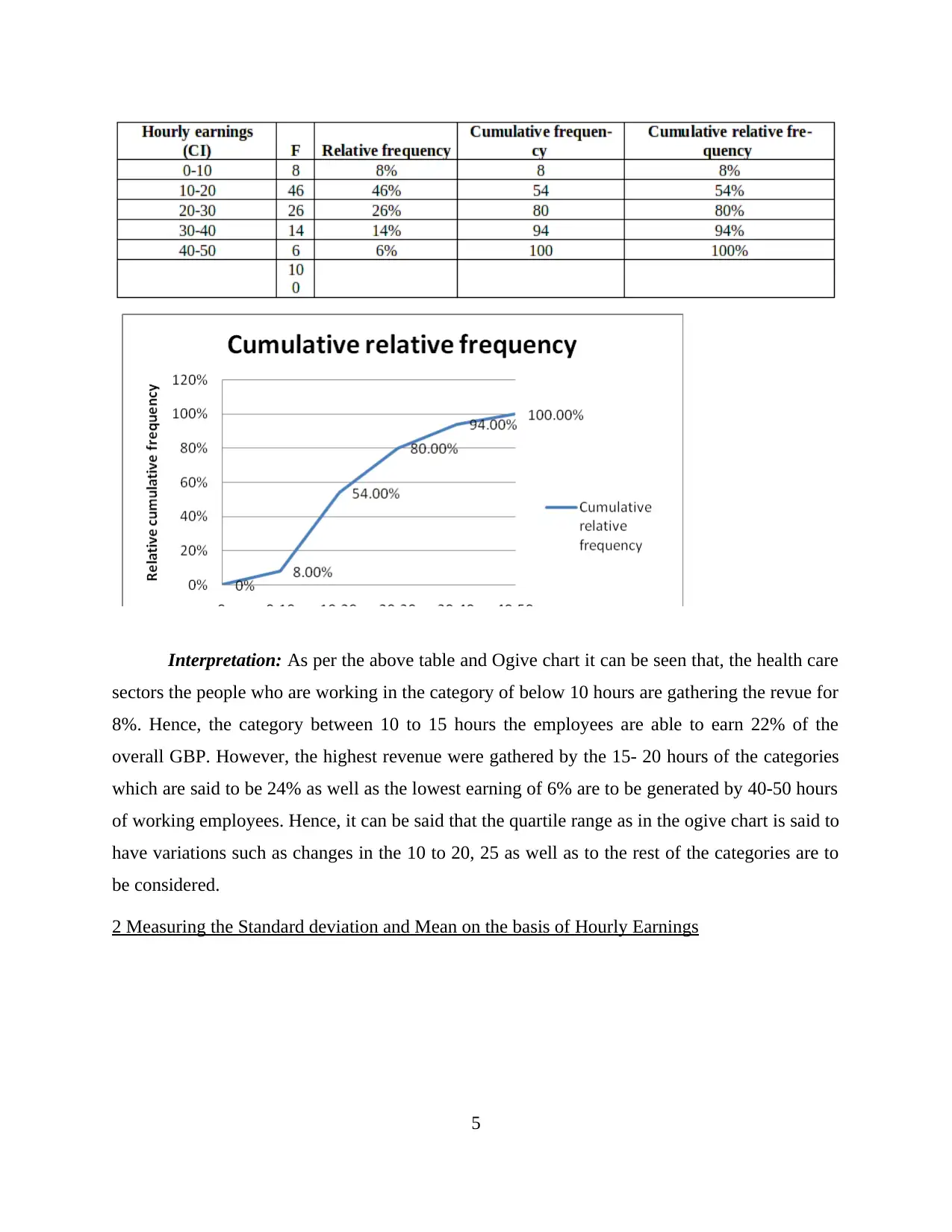
Interpretation: As per the above table and Ogive chart it can be seen that, the health care
sectors the people who are working in the category of below 10 hours are gathering the revue for
8%. Hence, the category between 10 to 15 hours the employees are able to earn 22% of the
overall GBP. However, the highest revenue were gathered by the 15- 20 hours of the categories
which are said to be 24% as well as the lowest earning of 6% are to be generated by 40-50 hours
of working employees. Hence, it can be said that the quartile range as in the ogive chart is said to
have variations such as changes in the 10 to 20, 25 as well as to the rest of the categories are to
be considered.
2 Measuring the Standard deviation and Mean on the basis of Hourly Earnings
5

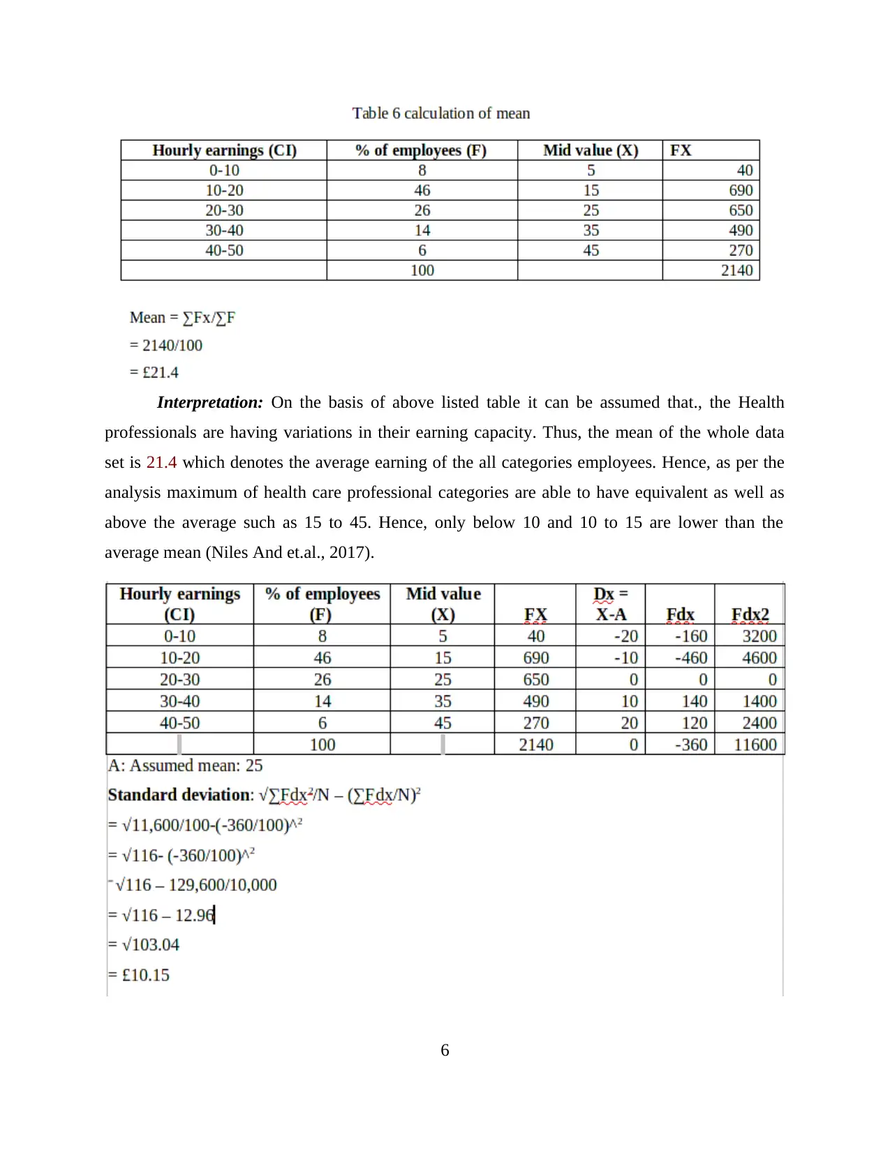
Interpretation: On the basis of above listed table it can be assumed that., the Health
professionals are having variations in their earning capacity. Thus, the mean of the whole data
set is 21.4 which denotes the average earning of the all categories employees. Hence, as per the
analysis maximum of health care professional categories are able to have equivalent as well as
above the average such as 15 to 45. Hence, only below 10 and 10 to 15 are lower than the
average mean (Niles And et.al., 2017).
6

Interpretation: As per the above analysis it can be said that, Standard deviation of such
data set is higher than the mean of the same. Hence, which indicates that, the low rate of mean
will affect the whole data analysis as well as to have better earning in the hourly basis there is
need to involve fewer employees on each hourly basis (Dula and et.al., 2016).
(B) Analysing the North East Health professionals as compared to South East.
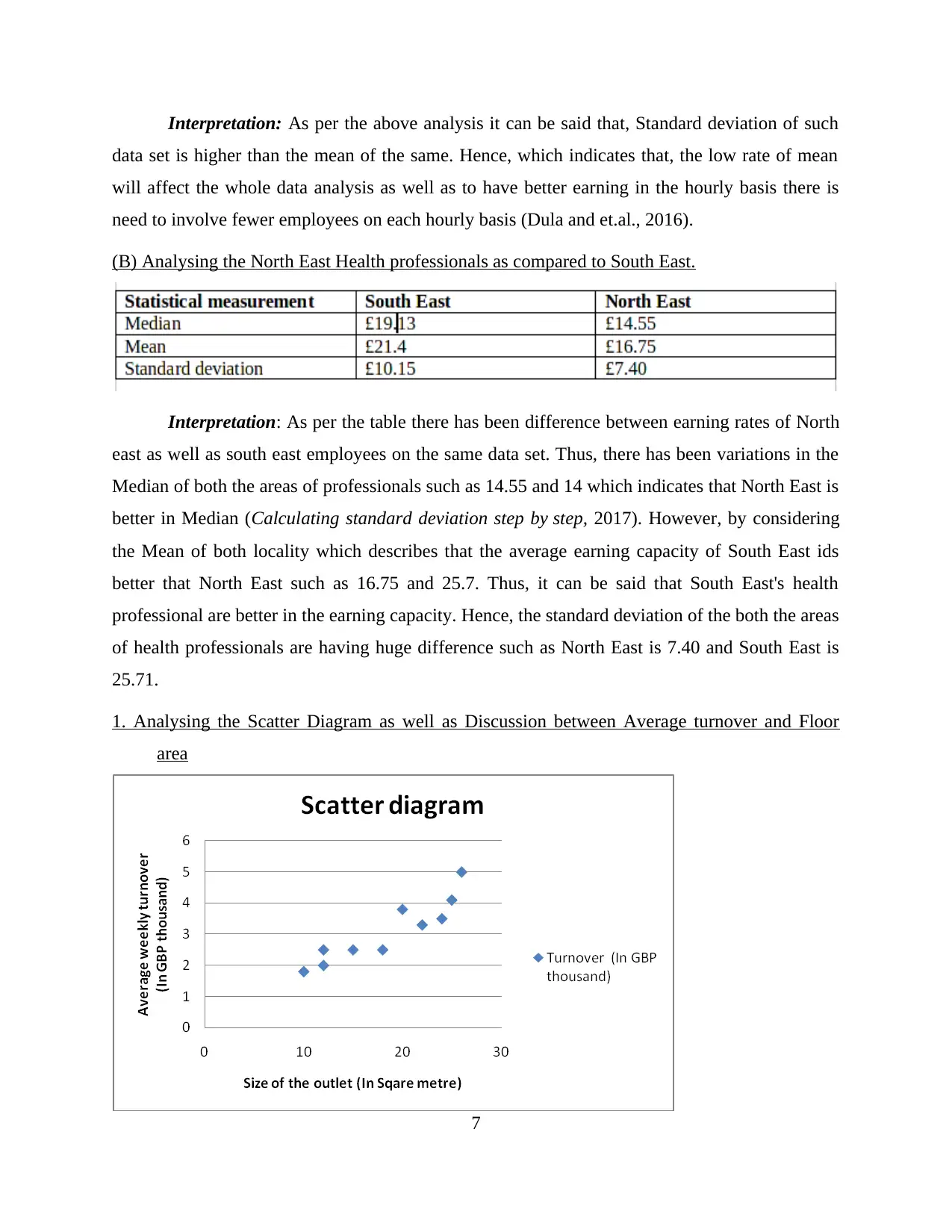
Interpretation: As per the table there has been difference between earning rates of North
east as well as south east employees on the same data set. Thus, there has been variations in the
Median of both the areas of professionals such as 14.55 and 14 which indicates that North East is
better in Median (Calculating standard deviation step by step, 2017). However, by considering
the Mean of both locality which describes that the average earning capacity of South East ids
better that North East such as 16.75 and 25.7. Thus, it can be said that South East's health
professional are better in the earning capacity. Hence, the standard deviation of the both the areas
of health professionals are having huge difference such as North East is 7.40 and South East is
25.71.
1. Analysing the Scatter Diagram as well as Discussion between Average turnover and Floor
area
7

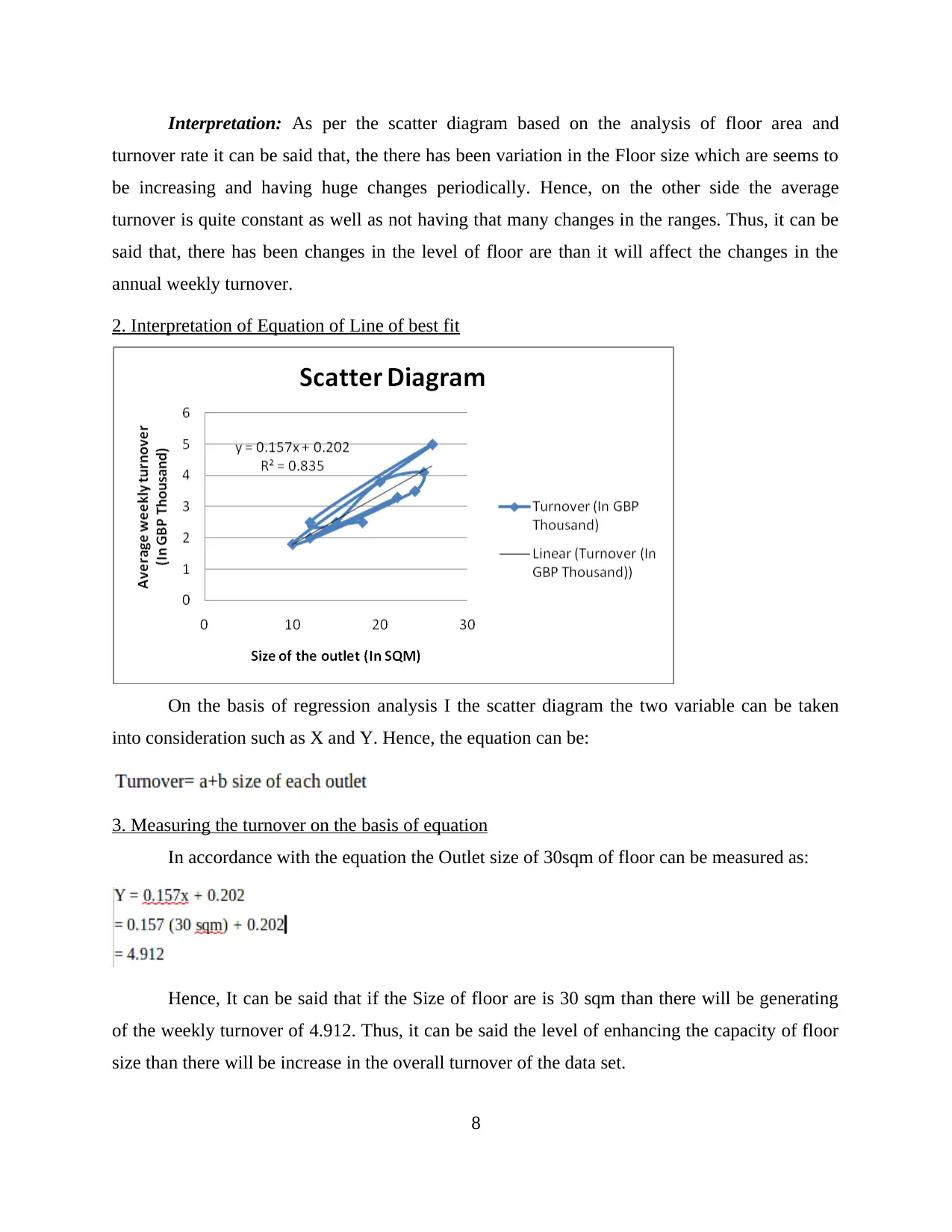
Interpretation: As per the scatter diagram based on the analysis of floor area and
turnover rate it can be said that, the there has been variation in the Floor size which are seems to
be increasing and having huge changes periodically. Hence, on the other side the average
turnover is quite constant as well as not having that many changes in the ranges. Thus, it can be
said that, there has been changes in the level of floor are than it will affect the changes in the
annual weekly turnover.
2. Interpretation of Equation of Line of best fit
On the basis of regression analysis I the scatter diagram the two variable can be taken
into consideration such as X and Y. Hence, the equation can be:
3. Measuring the turnover on the basis of equation
In accordance with the equation the Outlet size of 30sqm of floor can be measured as:
Hence, It can be said that if the Size of floor are is 30 sqm than there will be generating
of the weekly turnover of 4.912. Thus, it can be said the level of enhancing the capacity of floor
size than there will be increase in the overall turnover of the data set.
8

4. Measurement of regression and the correlation coefficient.
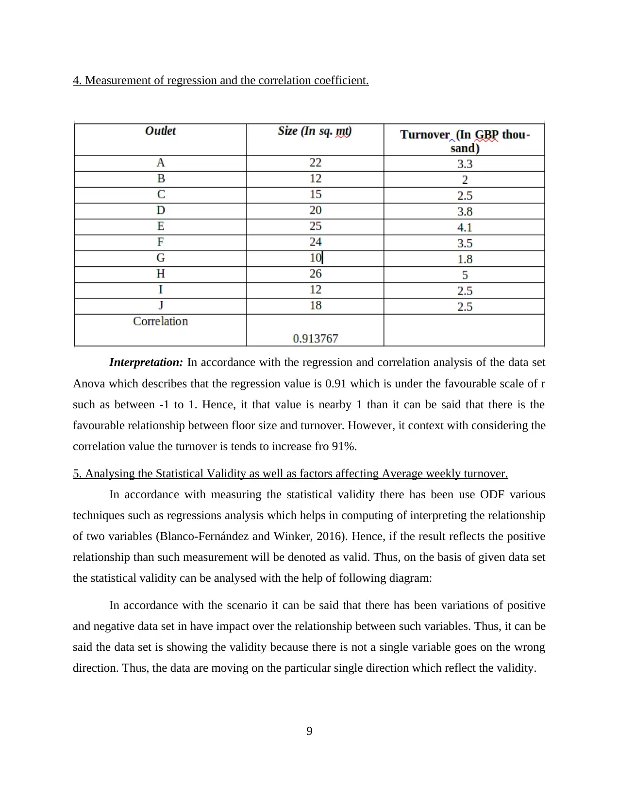
Interpretation: In accordance with the regression and correlation analysis of the data set
Anova which describes that the regression value is 0.91 which is under the favourable scale of r
such as between -1 to 1. Hence, it that value is nearby 1 than it can be said that there is the
favourable relationship between floor size and turnover. However, it context with considering the
correlation value the turnover is tends to increase fro 91%.
5. Analysing the Statistical Validity as well as factors affecting Average weekly turnover.
In accordance with measuring the statistical validity there has been use ODF various
techniques such as regressions analysis which helps in computing of interpreting the relationship
of two variables (Blanco-Fernández and Winker, 2016). Hence, if the result reflects the positive
relationship than such measurement will be denoted as valid. Thus, on the basis of given data set
the statistical validity can be analysed with the help of following diagram:
In accordance with the scenario it can be said that there has been variations of positive
and negative data set in have impact over the relationship between such variables. Thus, it can be
said the data set is showing the validity because there is not a single variable goes on the wrong
direction. Thus, the data are moving on the particular single direction which reflect the validity.
9

TASK 3
(B) Measuring the supply of olive oil bottles
1. Calculating the numbers of delivery made in each year
On the basis of given data set, it will be assumed that there has been delivery of various
numbers of olive oil bottles on which the entity has the 15% of market shares in such firm. Thus,
the numbers of delivery will be computed as 45000*15% = 67500 bottles.
2. Analysing the numbers of selling for olive oil in each Supply
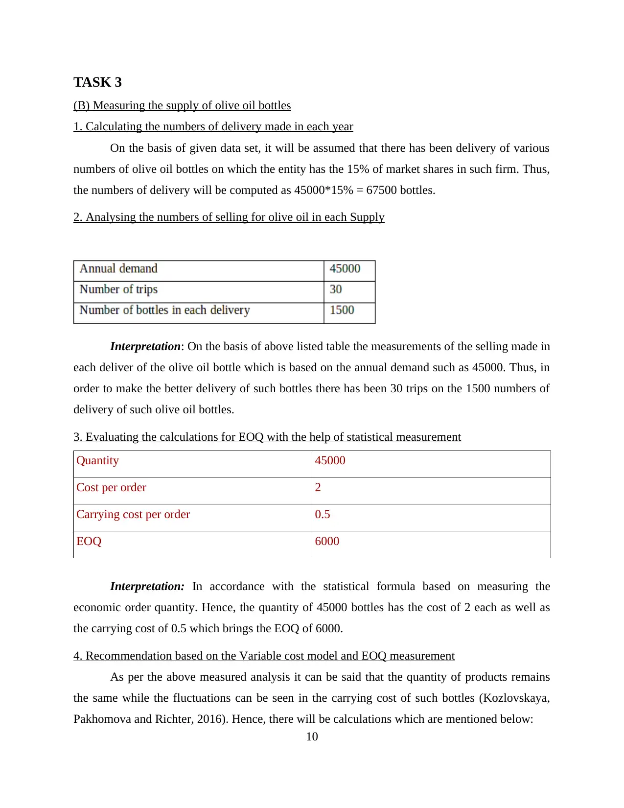
Interpretation: On the basis of above listed table the measurements of the selling made in
each deliver of the olive oil bottle which is based on the annual demand such as 45000. Thus, in
order to make the better delivery of such bottles there has been 30 trips on the 1500 numbers of
delivery of such olive oil bottles.
3. Evaluating the calculations for EOQ with the help of statistical measurement
Quantity 45000
Cost per order 2
Carrying cost per order 0.5
EOQ 6000
Interpretation: In accordance with the statistical formula based on measuring the
economic order quantity. Hence, the quantity of 45000 bottles has the cost of 2 each as well as
the carrying cost of 0.5 which brings the EOQ of 6000.
4. Recommendation based on the Variable cost model and EOQ measurement
As per the above measured analysis it can be said that the quantity of products remains
the same while the fluctuations can be seen in the carrying cost of such bottles (Kozlovskaya,
Pakhomova and Richter, 2016). Hence, there will be calculations which are mentioned below:
10

Interpretation: In accordance with the outcomes shown in the table there has been
variation in the carrying cost per bottle is fluctuating or changing but the quantity and the cost
per order remains the same. Thus, such as variation reflects in the difference between EOQ
outcomes. Hence, for the first order it is 600 and to the last order is results at 557.09.
TASK 4
1. Findings based on the data set in the task 2
Interpretation: on the basis of the data set provided in the task 2 the scatter diagram
facilitates the difference between floor area and average turnover. Thus, it can be said the
relationship between both the variable were tends to be measured as per the increase or decrease
in the floor size which will affect in increasing the volume of turnover.
11

2 Demonstrating the diagram on the basis of task 1
3 Presenting the diagram on the basis of data used in Task 2 in table 2
CONCLUSION
On the basis of above mentioned statistical analysis of various variables it can be said
that the to have the adequate information the statistical measurements is very helpful. Thus, the
mean, median and standard deviation measurement of the South East and North East health care
professionals facilitate the differences between their earning capacity. Hence, in context with
selling of the Olive Oil bottles which as variations In the carrying cost thus reflects the difference
12

in the outcomes of EOQ measurement. Further, it can be said in order to have better cost control
or analysis of capacity there is need to measure the outcomes with statistical methods.
13

REFERENCES
Books and Journals
Blanco-Fernández, A. and Winker, P., 2016. Data generation processes and statistical
management of interval data. AStA Advances in Statistical Analysis. 100(4). pp.475-494.
Dula, M. and et.al., 2016. Median and Mode Approximation for Skewed Unimodal Continuous
Distributions using Taylor Series Expansion.
Köhler, T., Landis, R. S. and Cortina, J. M., 2017. From the Editors: Establishing
Methodological Rigor in Quantitative Management Learning and Education Research: The
Role of Design, Statistical Methods, and Reporting Standards. Academy of Management
Learning & Education. 16(2). pp.173-192.
Kozlovskaya, N., Pakhomova, N. and Richter, K., 2016. The Optimal Disposal Rate for the
Extended EOQ Repair and Waste Disposal Model with Switching Costs. In Nachhaltiges
Entscheiden (pp. 549-568). Springer Fachmedien Wiesbaden.
Niles, A.N. And et.al., 2017. Advancing Personalized Medicine: Application of a Novel
Statistical Method to Identify Treatment Moderators in the Coordinated Anxiety Learning
and Management Study. Behavior Therapy. 48(4). pp.490-500.
Schmerler, E. and et.al., 2016. Experimental and numerical study of Sharp’s shadow zone
hypothesis on sand ripple wavelength. Aeolian Research. 22. pp.37-46.
Online
Calculating standard deviation step by step. 2017. [Online]. [Availabe through]
:<https://www.khanacademy.org/math/probability/data-distributions-a1/summarizing-
spread-distributions/a/calculating-standard-deviation-step-by-step>. [Accessed on 25th
October. 2017].
14