Statistics for Management: Income and Economic Analysis Report

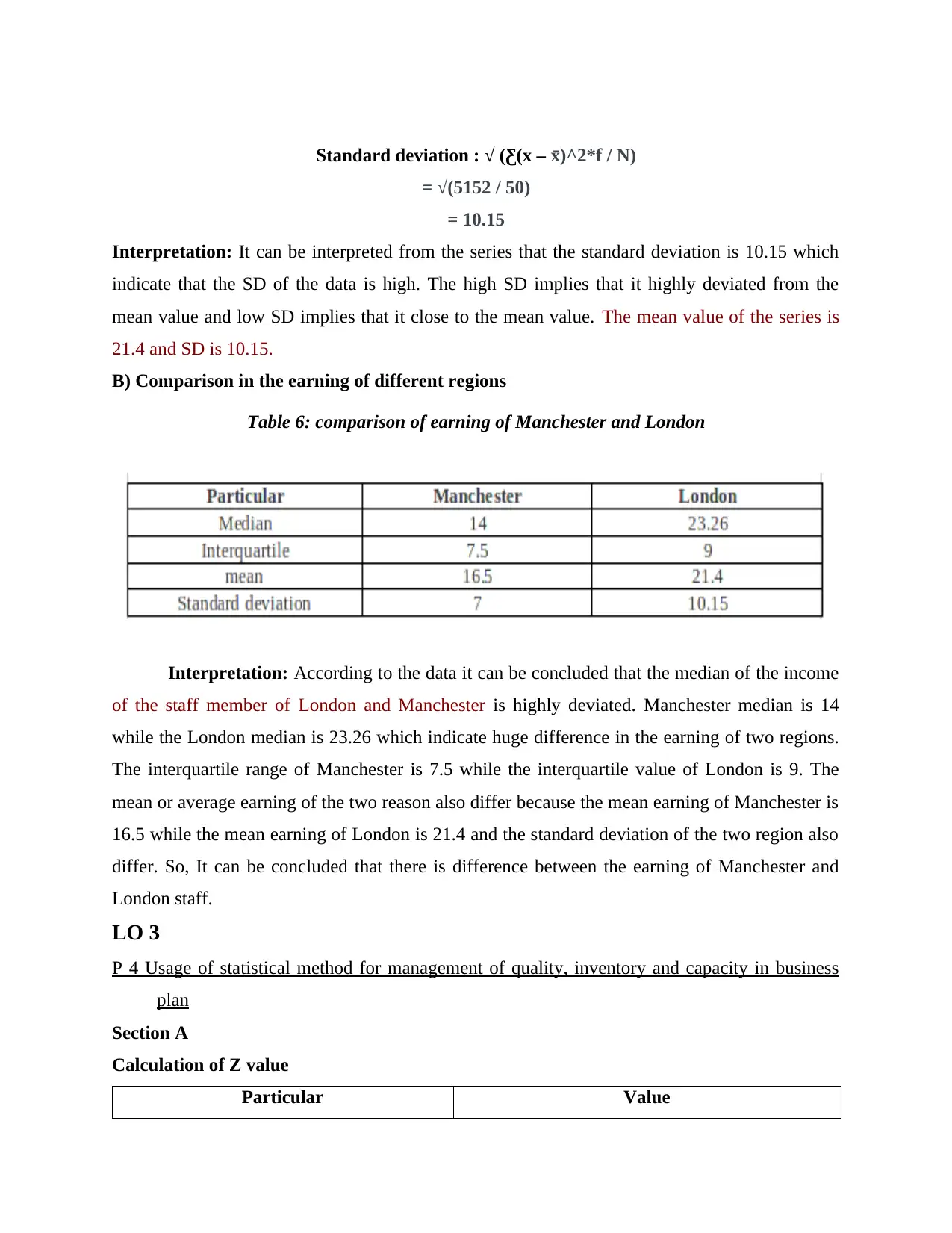
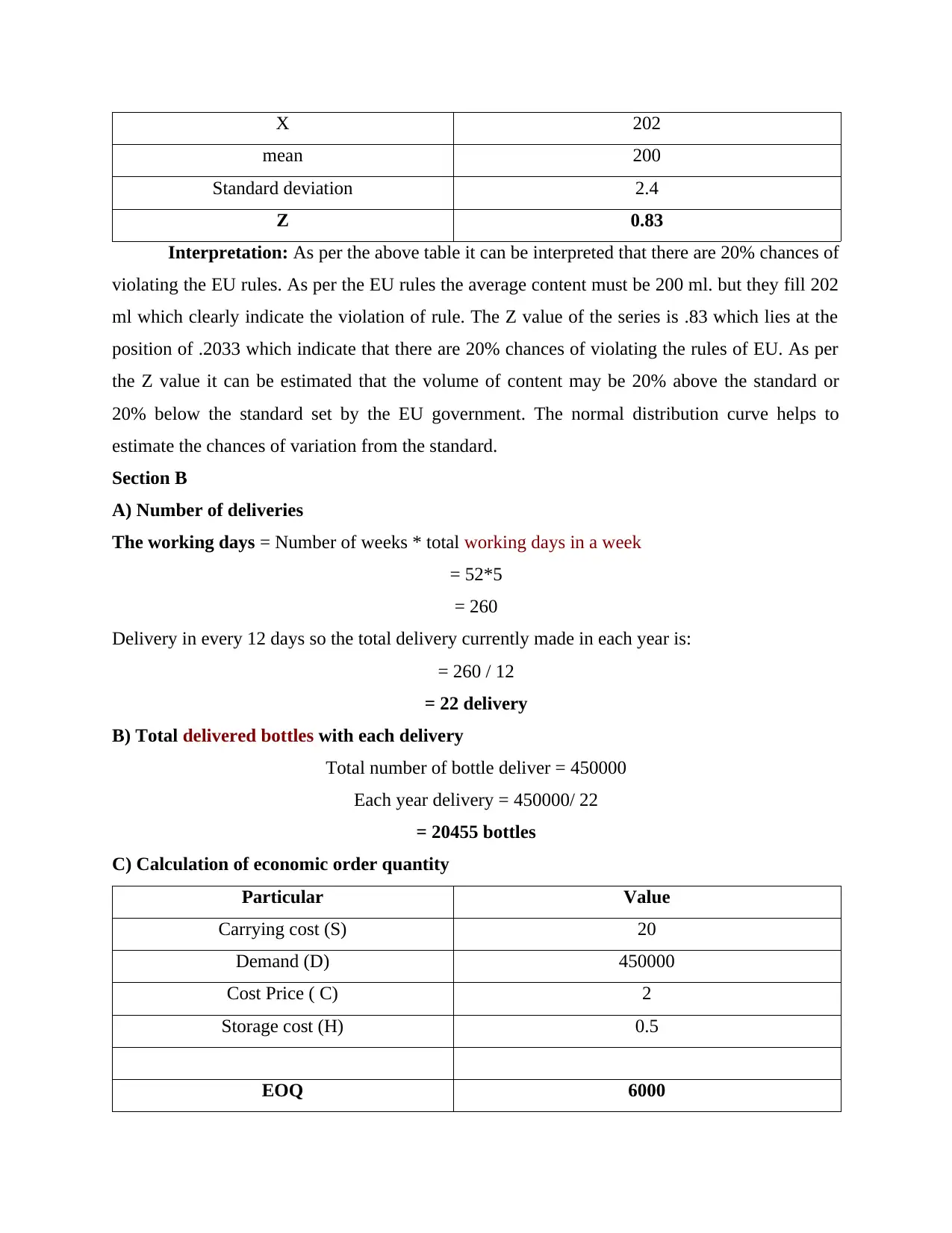
This report provides a comprehensive statistical analysis of income data, focusing on comparisons between public and private sector employees, income growth trends, and regional differences. It utilizes various statistical methods, including hypothesis testing, median, quartile, mean, and standard deviation calculations, to interpret the data. The report also explores the application of statistical techniques in business planning, such as the calculation of Economic Order Quantity (EOQ) for inventory management and Z-value calculation for quality control. Furthermore, the report incorporates the use of charts and tables for effective data presentation and communication of findings. Overall, the analysis aims to provide insights into income structures, economic trends, and the practical application of statistical tools in management decision-making.

STATISTICS FOR
MANAGEMENT

INTRODUCTION
Statistical analysis refers to a tool which helps the managers to make large quantitative
data into the understandable number to take effective and efficient decision on the basis of the
data. Statistical method are divided in two categories such as description method and inference
method. The report highlights the difference in the income of different sector employees. The
income growth rate explains the income structure across the different time period. It explains the
use central tendency method to compare the earning of different regions. The Ogive chart helps
to explain the relation in median and quartiles. It also explains the different statistical method
and their usage in business planning of the organization. It highlights the use of economic order
quantity for the effective production. The report also highlights the usage of charts for
communicating effective and efficient information.
LO 1
P 1 Different economic data and their presentation in graph and table format
A) Differences in the income structure of different sector employees from the different
published data
Null Hypothesis H0: There is no significance variances in the earning of men and women who
work in Public sector organization.
Alternative Hypothesis H1: There is significance variances in the earning of both men and
women sector who work in Public sector organization.
Table 1: Significance in the income of public sector employees
Interpretation: A hypothesis is used to create relation between two variables. The main
purpose of creating hypothesis is to identify the answers of different questions. According to the

calculation it can be summarized that the P value of the series is 1.35 which is larger than .05
value. It indicates that there is no significance difference in the variables or the income of the
employees who work in public sector (Gries, 2017). So, it doesn't require the alternative
hypothesis. The government provide various facilities to both men and women to equalize their
earning. The different laws and regulation force the public sector organization to pay equal
wages to same post employees that's why there is no significance difference in their earnings.
B) Comparison in the income of the employees of private sector organization from the
various source of data
Null hypothesis H0: There is no significance variances in the earning of private sector
employees.
Alternative hypothesis H1: There is significance variances in the earning of private sector
employees.
Table 2: Significance difference in the earning in private sector employees
Interpretation: According to the given data or calculation it can be summarized that P
value of the collected data or information is 2.16 which is greater than .05 value. It indicates that
null hypothesis should be accepted rather than the alternative hypothesis. The private sector
organization pay the employees on the basis of skills, knowledge, job role and their performance
rather than to pay the employees on the basis of gender or sex (Demirci and et.al., 2016). It
equalizes their earning and minimize the variance in their income. The equality act, employment
law also force them to pay equally to both men and women who work on the same post.

P 2 Different sector earnings by time chart method
Table 3: Annual income in public sector
According to the given data or information the income of public sector employees varies
as per the passage of time. It helps to identify the annual earning and the trend in income growth.
The annual earning of public sector employees is growing with no significance difference.
Table 4: Annual income in private sector
1
2
3
4
5
6
7
8
0
10000
20000
30000
40000
Men and women income in public sector

As per the given data it can be concluded that the income of private sector employees
varies according to the time period. It is used to identify the trend in their earning from the year
2009 to 2016. It helps to compare the income of the employees in different year and measure the
trend.
1
2
3
4
5
6
7
8
0
10000
20000
30000
40000
Men and women in private sector
Men private sector Women private sector

Growth rate of the employees of different sector
Interpretation: As per the data it can be identified that income of employees is increased
with the passage of time but the trend is not fixed (Davis and et.al., 2016). Sometimes the
earning of employees is grown rapidly and sometimes the trend of growth of earning is slow. As
per the above table in 2010 growth in the income of private sector men employees is 2% and in
public sector is -2%. According to the information the growth rate in private sector women
employees in 2010 is 4%. The above table present the growth in the earning in different years.
LO 2
P 3 Analysis and evaluation of different qualitative and quantitative data
A 1) Estimation of median and quartile of Leisure centre staff data

Median: It refers to the centre value of the given data set. It can be calculated by
different methods (Alan, 2016). For simple series it can be calculating by arranging the whole
series value in ascending and descending order than divide the total number of data by 2. In
frequency table the series value are already adjust in ascending and descending order. In the odd
number of series the median is the middle number or value but in the even number series the
median of the data is mean of two central values of the series.
Calculation of median for the frequency distribution series
The median of the series of data can be calculated by different method. For the frequency
distribution table it can b e calculated as follows:
1. Calculate the relative frequency value by dividing the frequency of the series from the
total number.
2. Calculate cumulative relative frequency by adding all the relative frequency value of the
series.
3. Divide the last cumulative frequency number by the value 2 to identify the hourly earning
series.
= N / 2
N = Total of frequency
= 50 / 2
= 25
4. Here selected series is 10 – 20 because the value 25 lies in the following series and than
insert the following formula to calculate the value of median.
= L / 2 + H / f [N / 2 – C]
L = Median class Lower limit
H = Median class Higher limit value
N = Total frequency value
C = Cumulative frequency value just before the median class series value
F = Corresponding frequency value of the middle class limit
5. Calculate the median of the data by inserting the formula
= 10 / 2 + 20 / 23 [50 / 2 – 4]
= 5 + 0.86 [21]

= 23.26
Interpretation: As per the above calculation it can be identified that the median of the series is
23.26 which indicate that
0 – 10 10 – 20 20 – 30 30 – 40 40 – 50
0
0.2
0.4
0.6
0.8
1
1.2
0.08
0.46
0.26
0.14
0.060.08
0.54
0.8
0.94 1
Ogive chart
The following chart present the relative frequency value and cumulative relative frequency value
of the set of data.
Calculation of quartile from the set of data
Quartile: It refers to the statistical data which divide the series into 4 equal part to
compare the performance or value in different time interval (Quartile. 2019). It is used to
measure the spread of value above and below the mean value by diving the whole range of data
in four equal data. The first quartile express the 25% of total range of data, second quartile
express 50%, third quartile present 75% and the forth quartile present 100%. It is mainly used to
calculate interquartile to identify the variability around the median value.
Particulars Value
1 Quartile 4
3 Quartile 13
Interquartile 9

The interquartile value can be calculated by getting the difference between the 3rd and 1st quartile.
Here the interquartile value is 9.
Interpretation: According to the following graph it can be identified that 1 quartile data
of the number of leisure central staff is 4 and the 3 quartile value of the total number of leisure
central staff is 13. It indicates that 25% of the range is 4 and 75% of the range value is 9.
A 2) Mean and standard deviation calculation
Mean calculation:
Arithmetic Mean = Ƹfx / Ƹf
= 1070 / 50
= 21.4
Interpretation: As per the above table the mean value of the series is 21.4 which indicates
average hourly earning of the leisure central staff is lie between 10 – 20 series because the mean
value of the series is 21.4.
Standard deviation calculation
Table 5: Presentation of standard deviation

Standard deviation : √ (Ƹ(x – x̄)^2*f / N)
= √(5152 / 50)
= 10.15
Interpretation: It can be interpreted from the series that the standard deviation is 10.15 which
indicate that the SD of the data is high. The high SD implies that it highly deviated from the
mean value and low SD implies that it close to the mean value. The mean value of the series is
21.4 and SD is 10.15.
B) Comparison in the earning of different regions
Table 6: comparison of earning of Manchester and London
Interpretation: According to the data it can be concluded that the median of the income
of the staff member of London and Manchester is highly deviated. Manchester median is 14
while the London median is 23.26 which indicate huge difference in the earning of two regions.
The interquartile range of Manchester is 7.5 while the interquartile value of London is 9. The
mean or average earning of the two reason also differ because the mean earning of Manchester is
16.5 while the mean earning of London is 21.4 and the standard deviation of the two region also
differ. So, It can be concluded that there is difference between the earning of Manchester and
London staff.
LO 3
P 4 Usage of statistical method for management of quality, inventory and capacity in business
plan
Section A
Calculation of Z value
Particular Value

X 202
mean 200
Standard deviation 2.4
Z 0.83
Interpretation: As per the above table it can be interpreted that there are 20% chances of
violating the EU rules. As per the EU rules the average content must be 200 ml. but they fill 202
ml which clearly indicate the violation of rule. The Z value of the series is .83 which lies at the
position of .2033 which indicate that there are 20% chances of violating the rules of EU. As per
the Z value it can be estimated that the volume of content may be 20% above the standard or
20% below the standard set by the EU government. The normal distribution curve helps to
estimate the chances of variation from the standard.
Section B
A) Number of deliveries
The working days = Number of weeks * total working days in a week
= 52*5
= 260
Delivery in every 12 days so the total delivery currently made in each year is:
= 260 / 12
= 22 delivery
B) Total delivered bottles with each delivery
Total number of bottle deliver = 450000
Each year delivery = 450000/ 22
= 20455 bottles
C) Calculation of economic order quantity
Particular Value
Carrying cost (S) 20
Demand (D) 450000
Cost Price ( C) 2
Storage cost (H) 0.5
EOQ 6000