Statistics for Management: Detailed Data Analysis and Report
VerifiedAdded on 2020/06/04
|17
|3736
|34
Report
AI Summary
This report provides a comprehensive statistical analysis for management purposes. It begins with an introduction to statistical tools and their applications, including mean, mode, median, standard deviation, and correlation. The report then delves into specific tasks, such as analyzing changes in gross annual earnings in the public and private sectors, calculating the gap between male and female earnings, and preparing ogives to represent cumulative frequencies. Further analysis includes calculating the mean and standard deviation from a given dataset, assessing the relationship between floor area and average weekly turnover using scatter diagrams and correlation coefficients, and determining the economic order quantity for a supplier. The report also includes the creation of line charts and scatter diagrams to visualize the data, and ultimately draws conclusions based on the statistical findings. The report utilizes various formulas and calculations to provide a detailed understanding of the data and its implications for management decision-making.

Statistics for management
Paraphrase This Document
Need a fresh take? Get an instant paraphrase of this document with our AI Paraphraser
Table of Contents
INTRODUCTION......................................................................................................................4
TASK 1......................................................................................................................................4
(a) Change in the gross annual earnings in the public and private sector since 2009 and
gap in male and female gross annual earnings.......................................................................4
TASK 2......................................................................................................................................6
Question1...............................................................................................................................6
(a) Preparation of Ogive and Calculation of mean and standard deviation......................6
(b) Assessing the difference between the results............................................................10
Question 2............................................................................................................................10
(a) Preparation of scatter diagram and discussion on the association of floor area and
average weekly turnover......................................................................................................10
(b) Equation for the line that is best fit for the scatter diagram......................................11
(c) Calculation of turnover using the equation of scatter diagram..................................11
(d) Computation of correlation coefficient r...................................................................11
(e) Ascertaining the validity of the statistics...................................................................12
TASK 3....................................................................................................................................13
(B) Understanding the supplying of local super market......................................................13
(c) Number of bottles delivered in each delivery............................................................13
(d) Computation of economic Order quantity (EOQ).....................................................13
(e) Computation of the cost of current ordering policy and comparison of it to EOQ...14
TASK 4....................................................................................................................................15
(a) Preparation of scatter diagram for size versus turnover............................................15
(b) Preparation of line chart which indicates male gross annual earnings for the public
from 2009 to 2016 ...............................................................................................................15
CONCLUSION........................................................................................................................16
REFERENCES.........................................................................................................................17
Table of Figures
Figure 1Annual gross earnings...................................................................................................3
Figure 2 Gap between male and females earnings.....................................................................4
Figure 3 Hourly earnings and percentage of employees............................................................5
Figure 4 less than and more than type of data............................................................................5
Figure 5 Ogive............................................................................................................................6
Figure 6 Cumulative frequency calculation...............................................................................6
Figure 7 Calculation of mean.....................................................................................................8
Figure 8 Calculation of Standard deviation...............................................................................8
Figure 9 Difference between the calculations............................................................................9
Figure 10 Scatter diagram........................................................................................................10
Figure 11Size and turnover......................................................................................................11
Figure 12 Size and turnover.....................................................................................................14
Figure 13 Scatter diagram........................................................................................................15
Figure 14 table for line chart....................................................................................................15
Figure 15 Line chart for males.................................................................................................15
⊘ This is a preview!⊘
Do you want full access?
Subscribe today to unlock all pages.
Trusted by 1+ million students worldwide
INTRODUCTION
Statistics is an important tool used in the companies to analyse the data set and reach
to an effective conclusion. The main and primary functions of statistics are, mean, mode,
median, standard deviation and correlation. It is a practice of collecting and analysing the
data set so that some information and knowledge can be developed out of the numbers. The
report discuses various factors of statistics and its application in the market in the practical
format. The report ponders on change in the gross annual earnings in public and private
sector through calculation of change in percentage. The preparation ogives and, line char and
scatter diagrams will be discussed with its usage (Rovai, Baker and Ponton, 2013). Economic
order quantity will also be calculated in such a manner so that supplier can get benefit out of
it. It will also discuss mean, mode, median and correlation calculation in order to better
analyse the data. In the end, scatter diagram will be created for size versus turnover and a line
chart will be produced for male gross annual earnings for the public from 2009 to 2016.
TASK 1
(a) Change in the gross annual earnings in the public and private sector since 2009 and gap in
male and female gross annual earnings
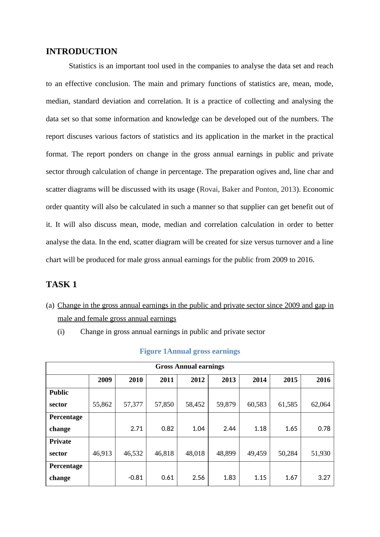
(i) Change in gross annual earnings in public and private sector
Figure 1Annual gross earnings
Gross Annual earnings
2009 2010 2011 2012 2013 2014 2015 2016
Public
sector 55,862 57,377 57,850 58,452 59,879 60,583 61,585 62,064
Percentage
change 2.71 0.82 1.04 2.44 1.18 1.65 0.78
Private
sector 46,913 46,532 46,818 48,018 48,899 49,459 50,284 51,930
Percentage
change -0.81 0.61 2.56 1.83 1.15 1.67 3.27
Statistics is an important tool used in the companies to analyse the data set and reach
to an effective conclusion. The main and primary functions of statistics are, mean, mode,
median, standard deviation and correlation. It is a practice of collecting and analysing the
data set so that some information and knowledge can be developed out of the numbers. The
report discuses various factors of statistics and its application in the market in the practical
format. The report ponders on change in the gross annual earnings in public and private
sector through calculation of change in percentage. The preparation ogives and, line char and
scatter diagrams will be discussed with its usage (Rovai, Baker and Ponton, 2013). Economic
order quantity will also be calculated in such a manner so that supplier can get benefit out of
it. It will also discuss mean, mode, median and correlation calculation in order to better
analyse the data. In the end, scatter diagram will be created for size versus turnover and a line
chart will be produced for male gross annual earnings for the public from 2009 to 2016.
TASK 1
(a) Change in the gross annual earnings in the public and private sector since 2009 and gap in
male and female gross annual earnings
(i) Change in gross annual earnings in public and private sector
Figure 1Annual gross earnings
Gross Annual earnings
2009 2010 2011 2012 2013 2014 2015 2016
Public
sector 55,862 57,377 57,850 58,452 59,879 60,583 61,585 62,064
Percentage
change 2.71 0.82 1.04 2.44 1.18 1.65 0.78
Private
sector 46,913 46,532 46,818 48,018 48,899 49,459 50,284 51,930
Percentage
change -0.81 0.61 2.56 1.83 1.15 1.67 3.27
Paraphrase This Document
Need a fresh take? Get an instant paraphrase of this document with our AI Paraphraser
From the data given, it can be analysed that there is a significant change in the gross
annual earnings of public sector percentage since 2009. The growth rate was decreased in the
initial year 2009 from 2.71% to 0.82 %. The growth rate further fluctuated in 2013 and
reached to 2.44%. However, it decreased again in 2016 and reached to 0.78% only in 2016.
From the percentage change analysis in private sector for gross annual earnings, it can
be interpreted that the growth rate was in negative in 2010. However, the rate steadily grew
and reached to 3,27% in 2016 which is higher than that of public sector.
From the above data , it can be assessed that the performance of the earnings of
private sector in comparison of the growth in the public sector.
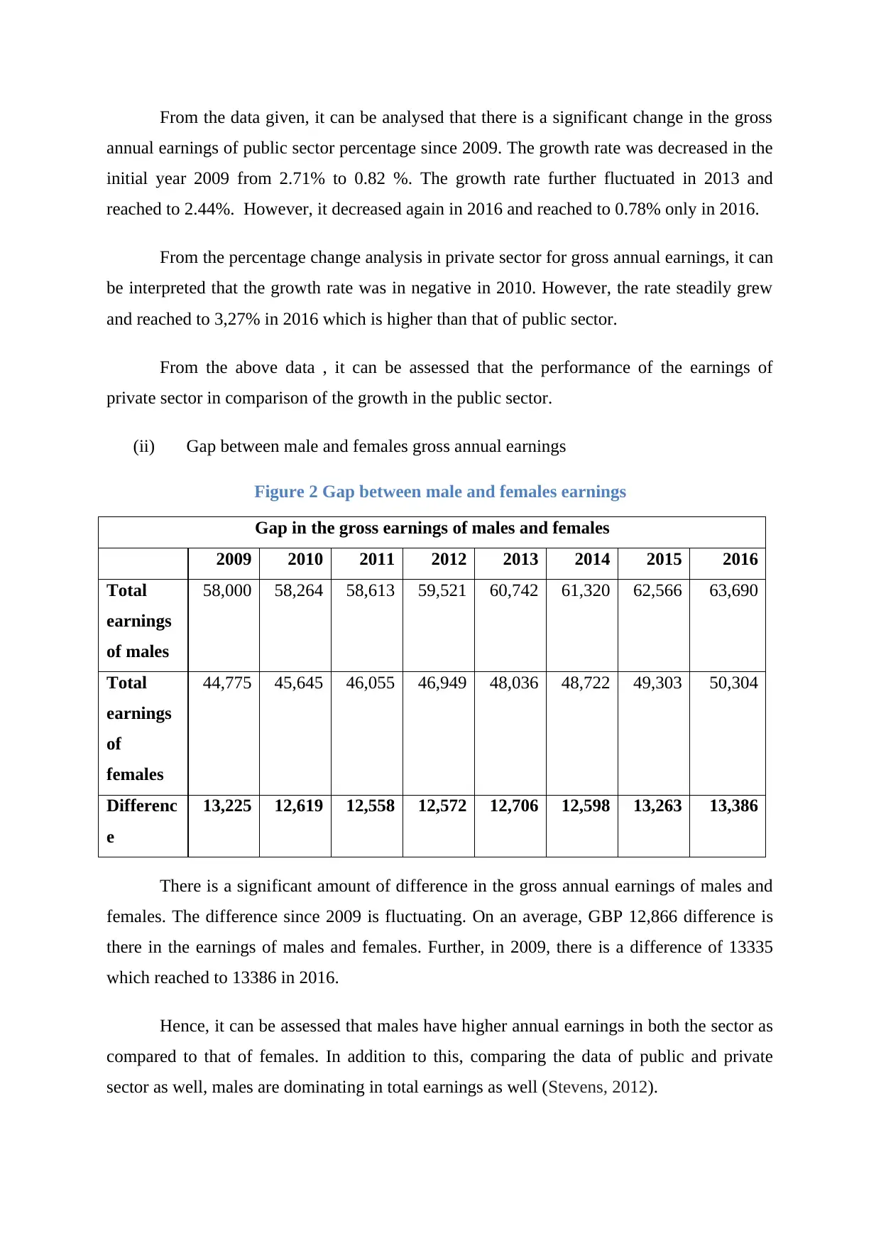
(ii) Gap between male and females gross annual earnings
Figure 2 Gap between male and females earnings
Gap in the gross earnings of males and females
2009 2010 2011 2012 2013 2014 2015 2016
Total
earnings
of males
58,000 58,264 58,613 59,521 60,742 61,320 62,566 63,690
Total
earnings
of
females
44,775 45,645 46,055 46,949 48,036 48,722 49,303 50,304
Differenc
e
13,225 12,619 12,558 12,572 12,706 12,598 13,263 13,386
There is a significant amount of difference in the gross annual earnings of males and
females. The difference since 2009 is fluctuating. On an average, GBP 12,866 difference is
there in the earnings of males and females. Further, in 2009, there is a difference of 13335
which reached to 13386 in 2016.
Hence, it can be assessed that males have higher annual earnings in both the sector as
compared to that of females. In addition to this, comparing the data of public and private
sector as well, males are dominating in total earnings as well (Stevens, 2012).
annual earnings of public sector percentage since 2009. The growth rate was decreased in the
initial year 2009 from 2.71% to 0.82 %. The growth rate further fluctuated in 2013 and
reached to 2.44%. However, it decreased again in 2016 and reached to 0.78% only in 2016.
From the percentage change analysis in private sector for gross annual earnings, it can
be interpreted that the growth rate was in negative in 2010. However, the rate steadily grew
and reached to 3,27% in 2016 which is higher than that of public sector.
From the above data , it can be assessed that the performance of the earnings of
private sector in comparison of the growth in the public sector.
(ii) Gap between male and females gross annual earnings
Figure 2 Gap between male and females earnings
Gap in the gross earnings of males and females
2009 2010 2011 2012 2013 2014 2015 2016
Total
earnings
of males
58,000 58,264 58,613 59,521 60,742 61,320 62,566 63,690
Total
earnings
of
females
44,775 45,645 46,055 46,949 48,036 48,722 49,303 50,304
Differenc
e
13,225 12,619 12,558 12,572 12,706 12,598 13,263 13,386
There is a significant amount of difference in the gross annual earnings of males and
females. The difference since 2009 is fluctuating. On an average, GBP 12,866 difference is
there in the earnings of males and females. Further, in 2009, there is a difference of 13335
which reached to 13386 in 2016.
Hence, it can be assessed that males have higher annual earnings in both the sector as
compared to that of females. In addition to this, comparing the data of public and private
sector as well, males are dominating in total earnings as well (Stevens, 2012).
TASK 2
Question1
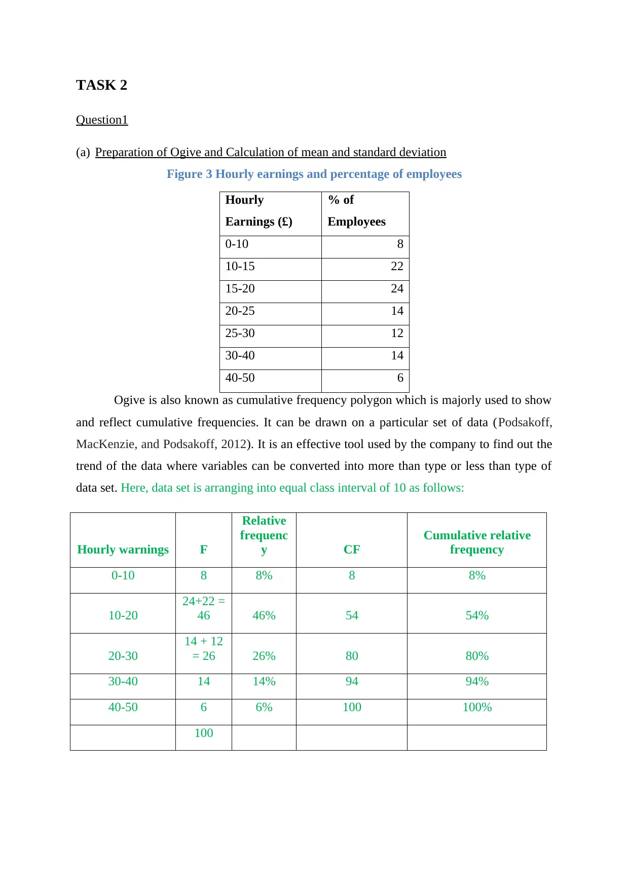
(a) Preparation of Ogive and Calculation of mean and standard deviation
Figure 3 Hourly earnings and percentage of employees
Hourly
Earnings (£)
% of
Employees
0-10 8
10-15 22
15-20 24
20-25 14
25-30 12
30-40 14
40-50 6
Ogive is also known as cumulative frequency polygon which is majorly used to show
and reflect cumulative frequencies. It can be drawn on a particular set of data (Podsakoff,
MacKenzie, and Podsakoff, 2012). It is an effective tool used by the company to find out the
trend of the data where variables can be converted into more than type or less than type of
data set. Here, data set is arranging into equal class interval of 10 as follows:
Hourly warnings F
Relative
frequenc
y CF
Cumulative relative
frequency
0-10 8 8% 8 8%
10-20
24+22 =
46 46% 54 54%
20-30
14 + 12
= 26 26% 80 80%
30-40 14 14% 94 94%
40-50 6 6% 100 100%
100
Question1
(a) Preparation of Ogive and Calculation of mean and standard deviation
Figure 3 Hourly earnings and percentage of employees
Hourly
Earnings (£)
% of
Employees
0-10 8
10-15 22
15-20 24
20-25 14
25-30 12
30-40 14
40-50 6
Ogive is also known as cumulative frequency polygon which is majorly used to show
and reflect cumulative frequencies. It can be drawn on a particular set of data (Podsakoff,
MacKenzie, and Podsakoff, 2012). It is an effective tool used by the company to find out the
trend of the data where variables can be converted into more than type or less than type of
data set. Here, data set is arranging into equal class interval of 10 as follows:
Hourly warnings F
Relative
frequenc
y CF
Cumulative relative
frequency
0-10 8 8% 8 8%
10-20
24+22 =
46 46% 54 54%
20-30
14 + 12
= 26 26% 80 80%
30-40 14 14% 94 94%
40-50 6 6% 100 100%
100
⊘ This is a preview!⊘
Do you want full access?
Subscribe today to unlock all pages.
Trusted by 1+ million students worldwide
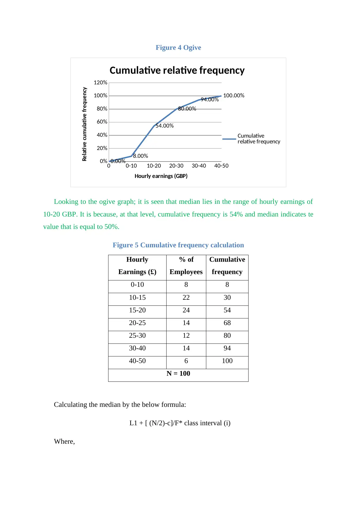
Figure 4 Ogive
0 0-10 10-20 20-30 30-40 40-50
0%
20%
40%
60%
80%
100%
120%
0.00% 8.00%
54.00%
80.00%
94.00% 100.00%
Cumulative relative frequency
Cumulative
relative frequency
Hourly earnings (GBP)
Relative cumulative frequency
Looking to the ogive graph; it is seen that median lies in the range of hourly earnings of
10-20 GBP. It is because, at that level, cumulative frequency is 54% and median indicates te
value that is equal to 50%.
Figure 5 Cumulative frequency calculation
Hourly
Earnings (£)
% of
Employees
Cumulative
frequency
0-10 8 8
10-15 22 30
15-20 24 54
20-25 14 68
25-30 12 80
30-40 14 94
40-50 6 100
N = 100
Calculating the median by the below formula:
L1 + [ (N/2)-c]/F* class interval (i)
Where,
Paraphrase This Document
Need a fresh take? Get an instant paraphrase of this document with our AI Paraphraser
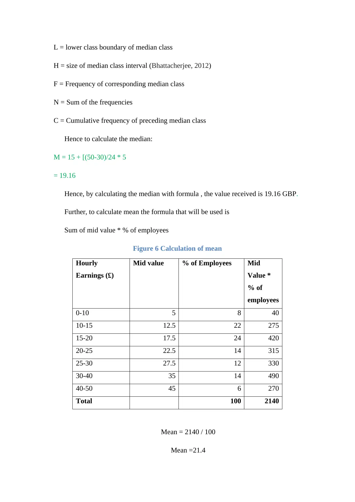
L = lower class boundary of median class
H = size of median class interval (Bhattacherjee, 2012)
F = Frequency of corresponding median class
N = Sum of the frequencies
C = Cumulative frequency of preceding median class
Hence to calculate the median:
M = 15 + [(50-30)/24 * 5
= 19.16
Hence, by calculating the median with formula , the value received is 19.16 GBP.
Further, to calculate mean the formula that will be used is
Sum of mid value * % of employees
Figure 6 Calculation of mean
Hourly
Earnings (£)
Mid value % of Employees Mid
Value *
% of
employees
0-10 5 8 40
10-15 12.5 22 275
15-20 17.5 24 420
20-25 22.5 14 315
25-30 27.5 12 330
30-40 35 14 490
40-50 45 6 270
Total 100 2140
Mean = 2140 / 100
Mean =21.4
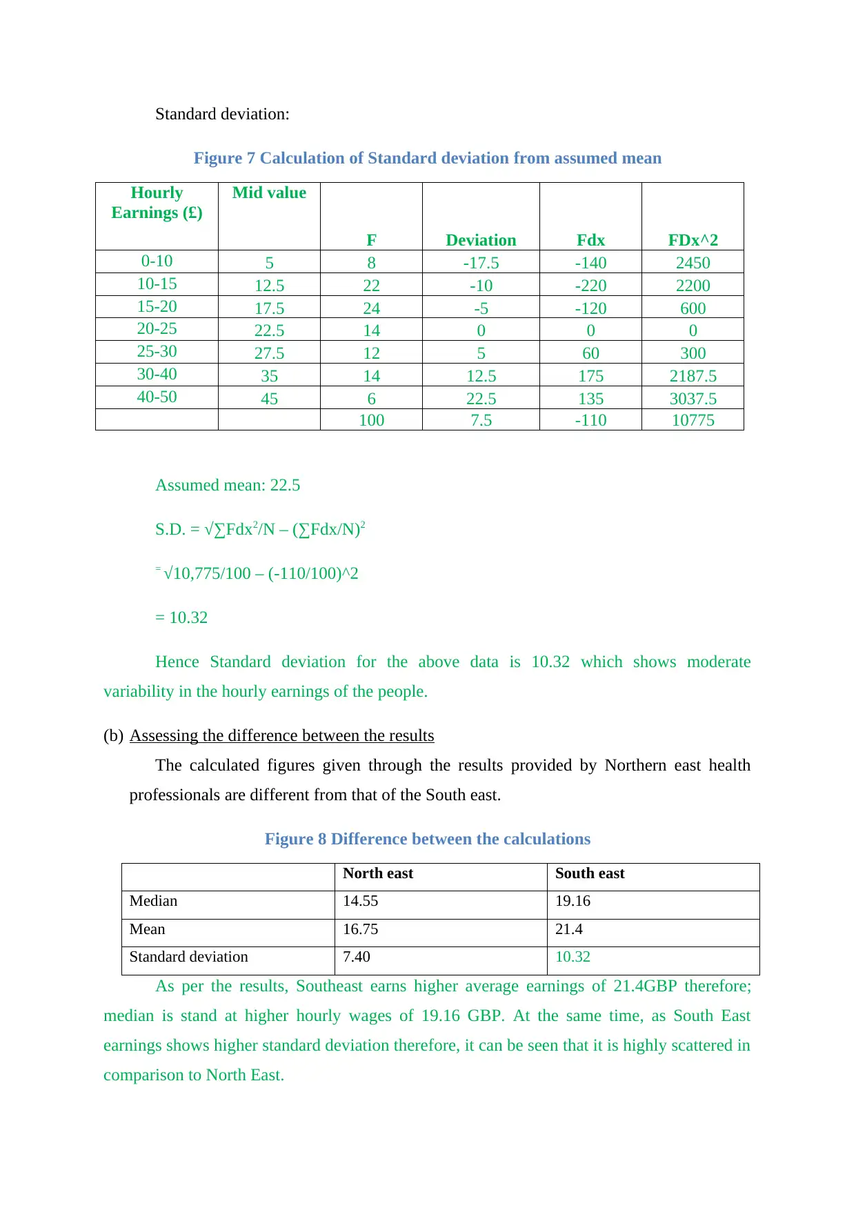
Standard deviation:
Figure 7 Calculation of Standard deviation from assumed mean
Hourly
Earnings (£)
Mid value
F Deviation Fdx FDx^2
0-10 5 8 -17.5 -140 2450
10-15 12.5 22 -10 -220 2200
15-20 17.5 24 -5 -120 600
20-25 22.5 14 0 0 0
25-30 27.5 12 5 60 300
30-40 35 14 12.5 175 2187.5
40-50 45 6 22.5 135 3037.5
100 7.5 -110 10775
Assumed mean: 22.5
S.D. = √∑Fdx2/N – (∑Fdx/N)2
= √10,775/100 – (-110/100)^2
= 10.32
Hence Standard deviation for the above data is 10.32 which shows moderate
variability in the hourly earnings of the people.
(b) Assessing the difference between the results
The calculated figures given through the results provided by Northern east health
professionals are different from that of the South east.
Figure 8 Difference between the calculations
North east South east
Median 14.55 19.16
Mean 16.75 21.4
Standard deviation 7.40 10.32
As per the results, Southeast earns higher average earnings of 21.4GBP therefore;
median is stand at higher hourly wages of 19.16 GBP. At the same time, as South East
earnings shows higher standard deviation therefore, it can be seen that it is highly scattered in
comparison to North East.
⊘ This is a preview!⊘
Do you want full access?
Subscribe today to unlock all pages.
Trusted by 1+ million students worldwide
Question 2
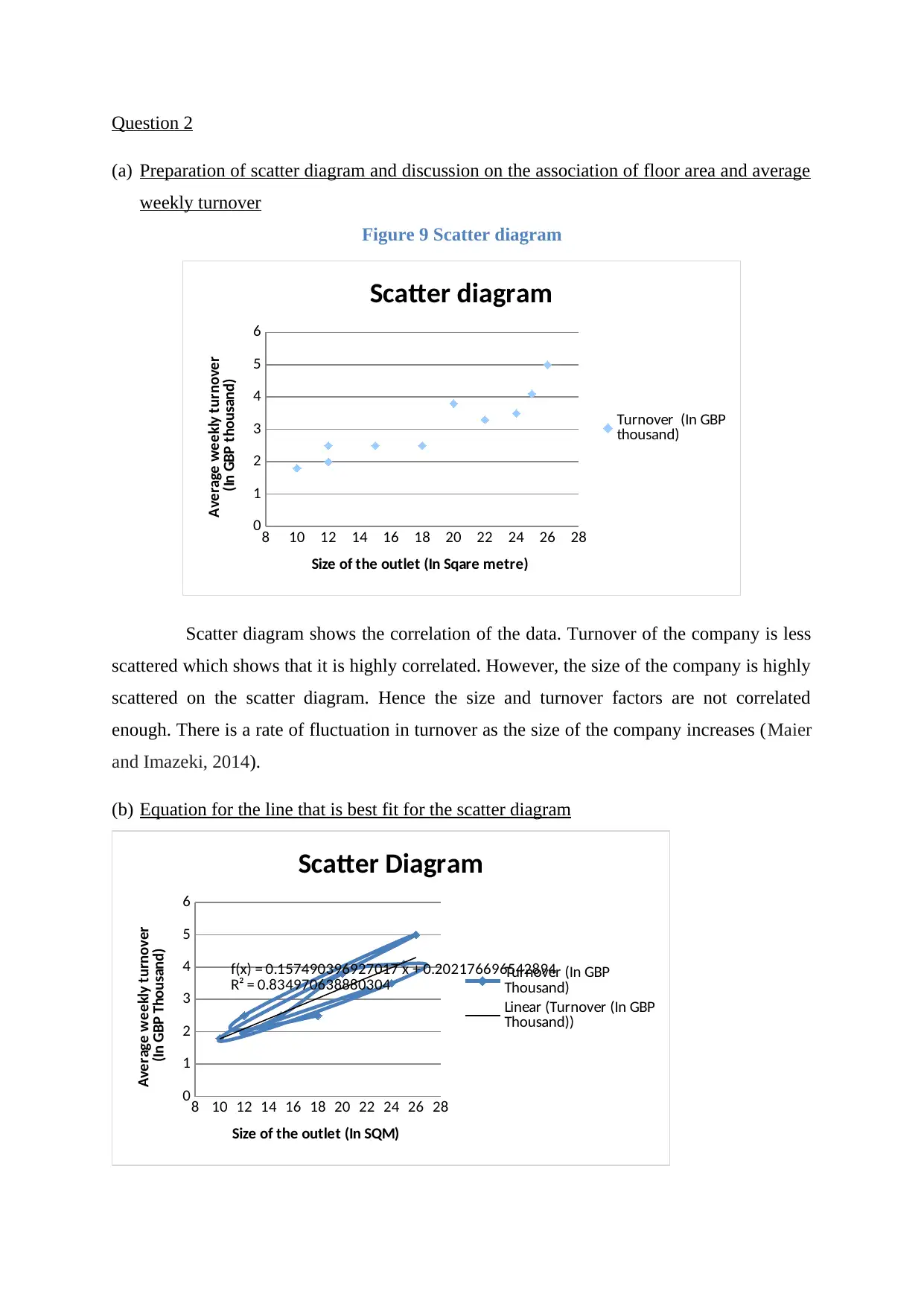
(a) Preparation of scatter diagram and discussion on the association of floor area and average
weekly turnover
Figure 9 Scatter diagram
8 10 12 14 16 18 20 22 24 26 28
0
1
2
3
4
5
6
Scatter diagram
Turnover (In GBP
thousand)
Size of the outlet (In Sqare metre)
Average weekly turnover
(In GBP thousand)
Scatter diagram shows the correlation of the data. Turnover of the company is less
scattered which shows that it is highly correlated. However, the size of the company is highly
scattered on the scatter diagram. Hence the size and turnover factors are not correlated
enough. There is a rate of fluctuation in turnover as the size of the company increases (Maier
and Imazeki, 2014).
(b) Equation for the line that is best fit for the scatter diagram
8 10 12 14 16 18 20 22 24 26 28
0
1
2
3
4
5
6
f(x) = 0.157490396927017 x + 0.202176696542894
R² = 0.834970638880304
Scatter Diagram
Turnover (In GBP
Thousand)
Linear (Turnover (In GBP
Thousand))
Size of the outlet (In SQM)
Average weekly turnover
(In GBP Thousand)
Paraphrase This Document
Need a fresh take? Get an instant paraphrase of this document with our AI Paraphraser
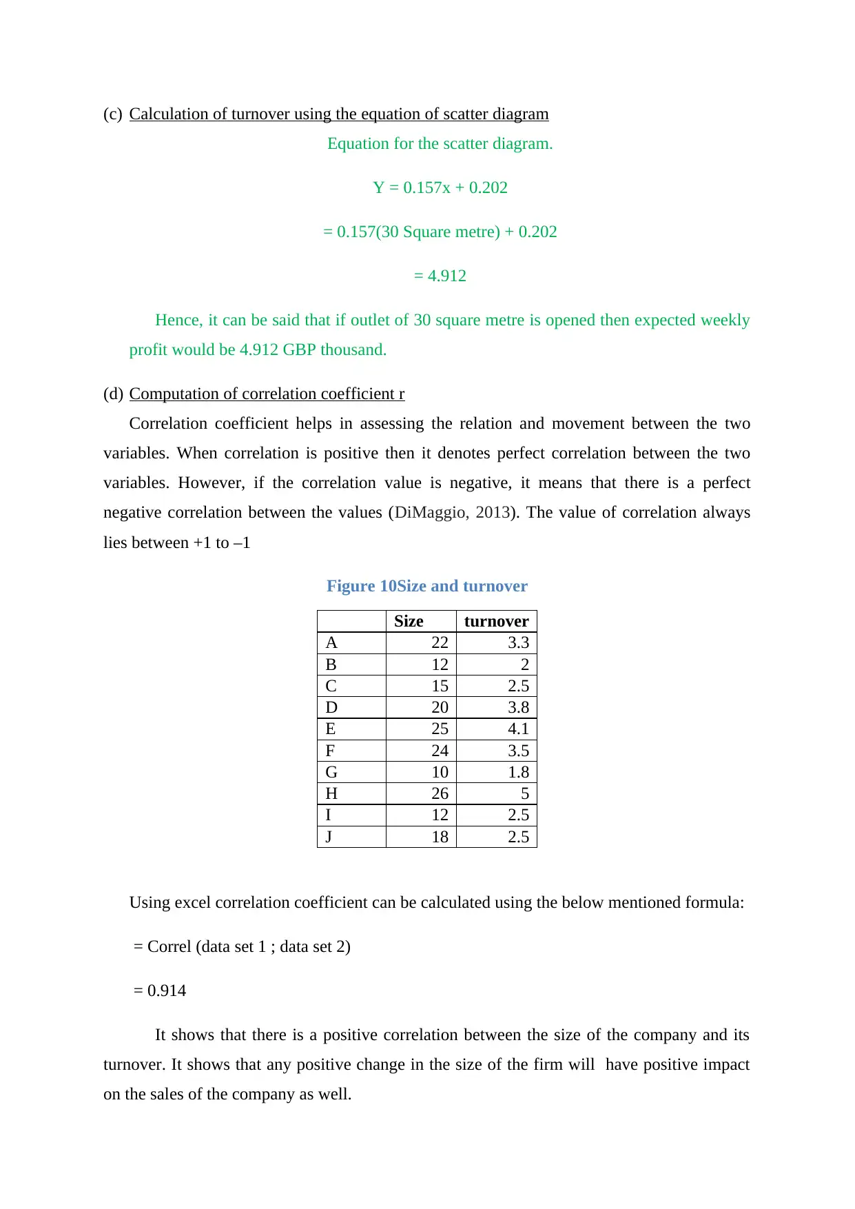
(c) Calculation of turnover using the equation of scatter diagram
Equation for the scatter diagram.
Y = 0.157x + 0.202
= 0.157(30 Square metre) + 0.202
= 4.912
Hence, it can be said that if outlet of 30 square metre is opened then expected weekly
profit would be 4.912 GBP thousand.
(d) Computation of correlation coefficient r
Correlation coefficient helps in assessing the relation and movement between the two
variables. When correlation is positive then it denotes perfect correlation between the two
variables. However, if the correlation value is negative, it means that there is a perfect
negative correlation between the values (DiMaggio, 2013). The value of correlation always
lies between +1 to –1
Figure 10Size and turnover
Size turnover
A 22 3.3
B 12 2
C 15 2.5
D 20 3.8
E 25 4.1
F 24 3.5
G 10 1.8
H 26 5
I 12 2.5
J 18 2.5
Using excel correlation coefficient can be calculated using the below mentioned formula:
= Correl (data set 1 ; data set 2)
= 0.914
It shows that there is a positive correlation between the size of the company and its
turnover. It shows that any positive change in the size of the firm will have positive impact
on the sales of the company as well.
(e) Ascertaining the validity of the statistics
The statistics and data that have been calculated are valid enough as all the authenticated
formulas for co efficient correlation are being used. The analysis also helps in predicting the
future as well (Rossi, Wright and Anderson, 2013). Further, it is important to rely on the data
of only correlation to reach to the results. Hence, it is important for the analyst to analyse the
data of mean, mode, median, and other important factors of statistics to draw out effective
and efficient conclusion of the data. The two other factors that could affect the average
weekly turnover are as follows:
Profits of the company: The profits that have been earned by the company helps in
determining the financial position of the company. It is difficult to ascertain the
position with only the turnover factor . Further, it also helps in assessing how much
percentage of discount have been provided to the customers in order to increase the
sales (Sovacool, 2014).
Cost of goods sold and other expenses: It is important to assess the cost of goods
sold and other expenses that have not been consider by the analysts to draw out the
result and that could have affected the average turnover of the company. Further, any
increase in any of the cost can reduce the profits of the company further impacting the
turnover of the business as well (Brown, 2013). An increase in the market price of the
product will also affect the current pricing policies increasing the turnover but not the
profits to that extend. Hence, these factors are important for the company to consider.
Had the researcher considered al the important factor while making the judgement for
the company, it could have been proved to be beneficial. Hence the statistics may not be
considered as authenticated as just on the basis of correlation, the data can not be
considered as reliable. It is important for the researcher to calculate, mean, mode , median
, standard deviation , for the data to find its authenticity and consider the above
mentioned factors as well (Alchon, 2014).
TASK 3
(B) Understanding the supplying of local super market
The number of deliveries made in the current year ca be calculated as below:
= 360 / 12
⊘ This is a preview!⊘
Do you want full access?
Subscribe today to unlock all pages.
Trusted by 1+ million students worldwide
1 out of 17
Related Documents


Your All-in-One AI-Powered Toolkit for Academic Success.
+13062052269
info@desklib.com
Available 24*7 on WhatsApp / Email
![[object Object]](/_next/static/media/star-bottom.7253800d.svg)
Unlock your academic potential
Copyright © 2020–2025 A2Z Services. All Rights Reserved. Developed and managed by ZUCOL.