Analyzing Statistical Data for Managerial Decision Making

The assignment 'Statistics for Managerial Decisions' is a comprehensive exploration of applying statistical techniques to solve real-world business problems. It includes the creation and interpretation of stem and leaf plots, calculation of probabilities in different contexts such as household distributions ...Read More

Running Head: STATISTICS FOR MANAGERIAL DECISIONS
Statistics for Managerial Decisions
Name of the Student
Name of the University
Author Note

1STATISTICS FOR MANAGERIAL DECISIONS
Answer 1
Part A
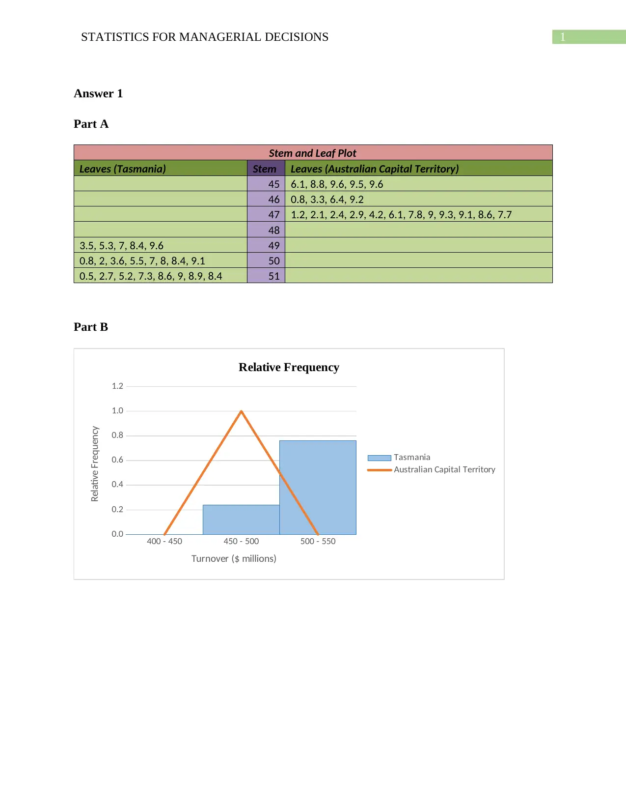
Stem and Leaf Plot
Leaves (Tasmania) Stem Leaves (Australian Capital Territory)
45 6.1, 8.8, 9.6, 9.5, 9.6
46 0.8, 3.3, 6.4, 9.2
47 1.2, 2.1, 2.4, 2.9, 4.2, 6.1, 7.8, 9, 9.3, 9.1, 8.6, 7.7
48
3.5, 5.3, 7, 8.4, 9.6 49
0.8, 2, 3.6, 5.5, 7, 8, 8.4, 9.1 50
0.5, 2.7, 5.2, 7.3, 8.6, 9, 8.9, 8.4 51
Part B
400 - 450 450 - 500 500 - 550
0.0
0.2
0.4
0.6
0.8
1.0
1.2
Relative Frequency
Tasmania
Australian Capital Territory
Turnover ($ millions)
Relative Frequency

2STATISTICS FOR MANAGERIAL DECISIONS
Part C
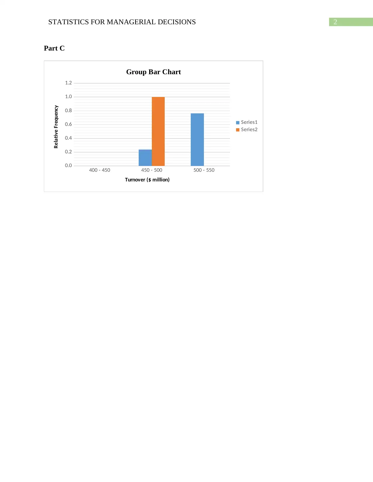
400 - 450 450 - 500 500 - 550
0.0
0.2
0.4
0.6
0.8
1.0
1.2
Group Bar Chart
Series1
Series2
Turnover ($ million)
Relative Frequency

3STATISTICS FOR MANAGERIAL DECISIONS
Answer 2
Part A
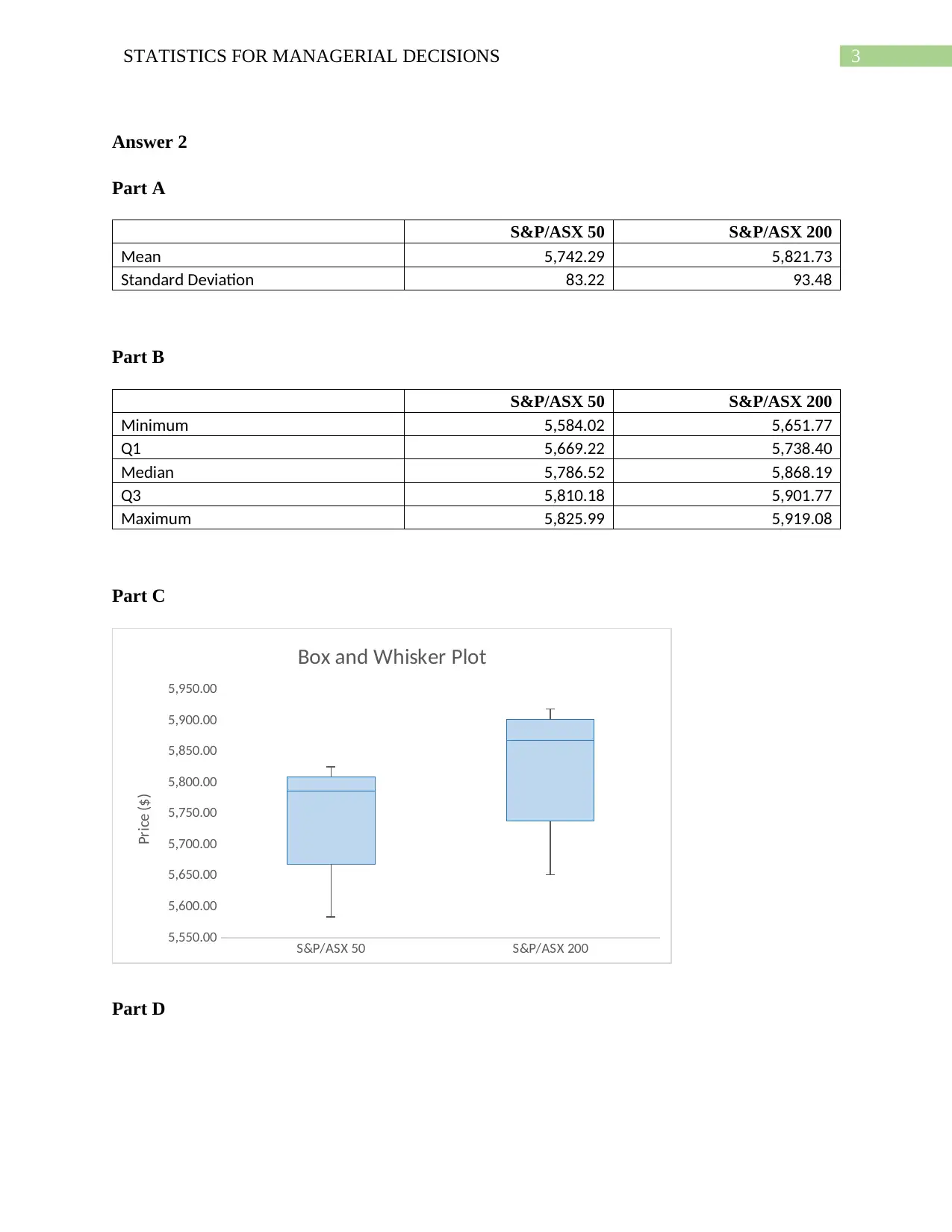
S&P/ASX 50 S&P/ASX 200
Mean 5,742.29 5,821.73
Standard Deviation 83.22 93.48
Part B
S&P/ASX 50 S&P/ASX 200
Minimum 5,584.02 5,651.77
Q1 5,669.22 5,738.40
Median 5,786.52 5,868.19
Q3 5,810.18 5,901.77
Maximum 5,825.99 5,919.08
Part C
S&P/ASX 50 S&P/ASX 200
5,550.00
5,600.00
5,650.00
5,700.00
5,750.00
5,800.00
5,850.00
5,900.00
5,950.00
Box and Whisker Plot
Price ($)
Part D

4STATISTICS FOR MANAGERIAL DECISIONS
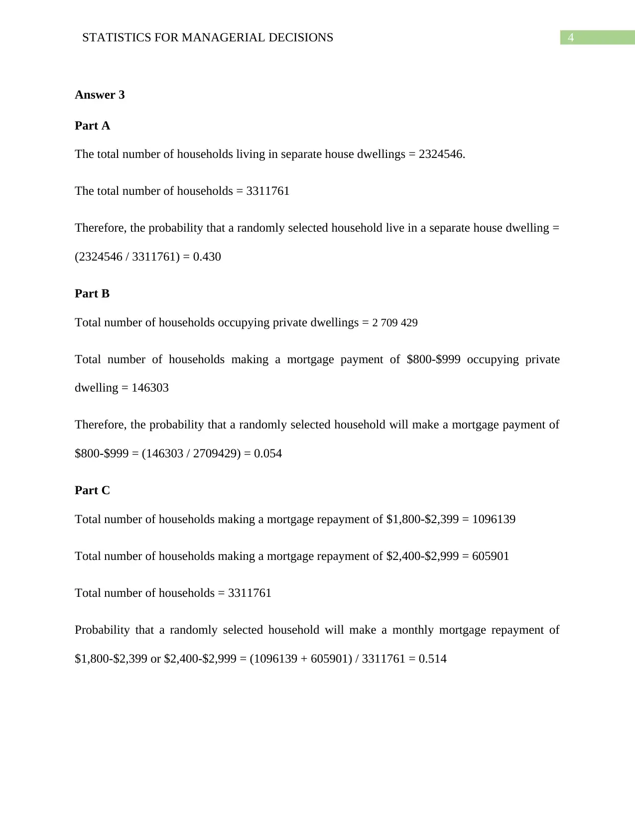
Answer 3
Part A
The total number of households living in separate house dwellings = 2324546.
The total number of households = 3311761
Therefore, the probability that a randomly selected household live in a separate house dwelling =
(2324546 / 3311761) = 0.430
Part B
Total number of households occupying private dwellings = 2 709 429
Total number of households making a mortgage payment of $800-$999 occupying private
dwelling = 146303
Therefore, the probability that a randomly selected household will make a mortgage payment of
$800-$999 = (146303 / 2709429) = 0.054
Part C
Total number of households making a mortgage repayment of $1,800-$2,399 = 1096139
Total number of households making a mortgage repayment of $2,400-$2,999 = 605901
Total number of households = 3311761
Probability that a randomly selected household will make a monthly mortgage repayment of
$1,800-$2,399 or $2,400-$2,999 = (1096139 + 605901) / 3311761 = 0.514

5STATISTICS FOR MANAGERIAL DECISIONS
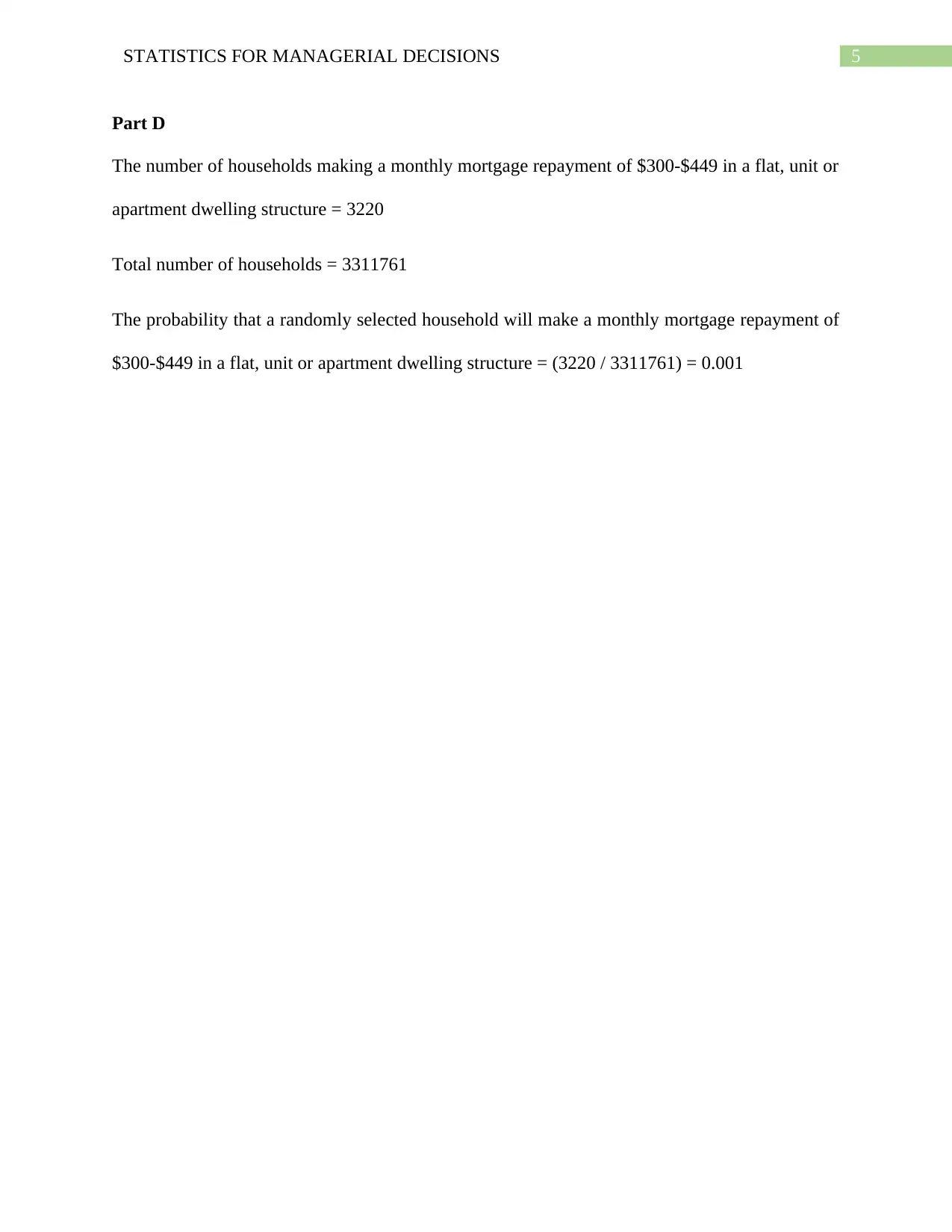
Part D
The number of households making a monthly mortgage repayment of $300-$449 in a flat, unit or
apartment dwelling structure = 3220
Total number of households = 3311761
The probability that a randomly selected household will make a monthly mortgage repayment of
$300-$449 in a flat, unit or apartment dwelling structure = (3220 / 3311761) = 0.001

6STATISTICS FOR MANAGERIAL DECISIONS
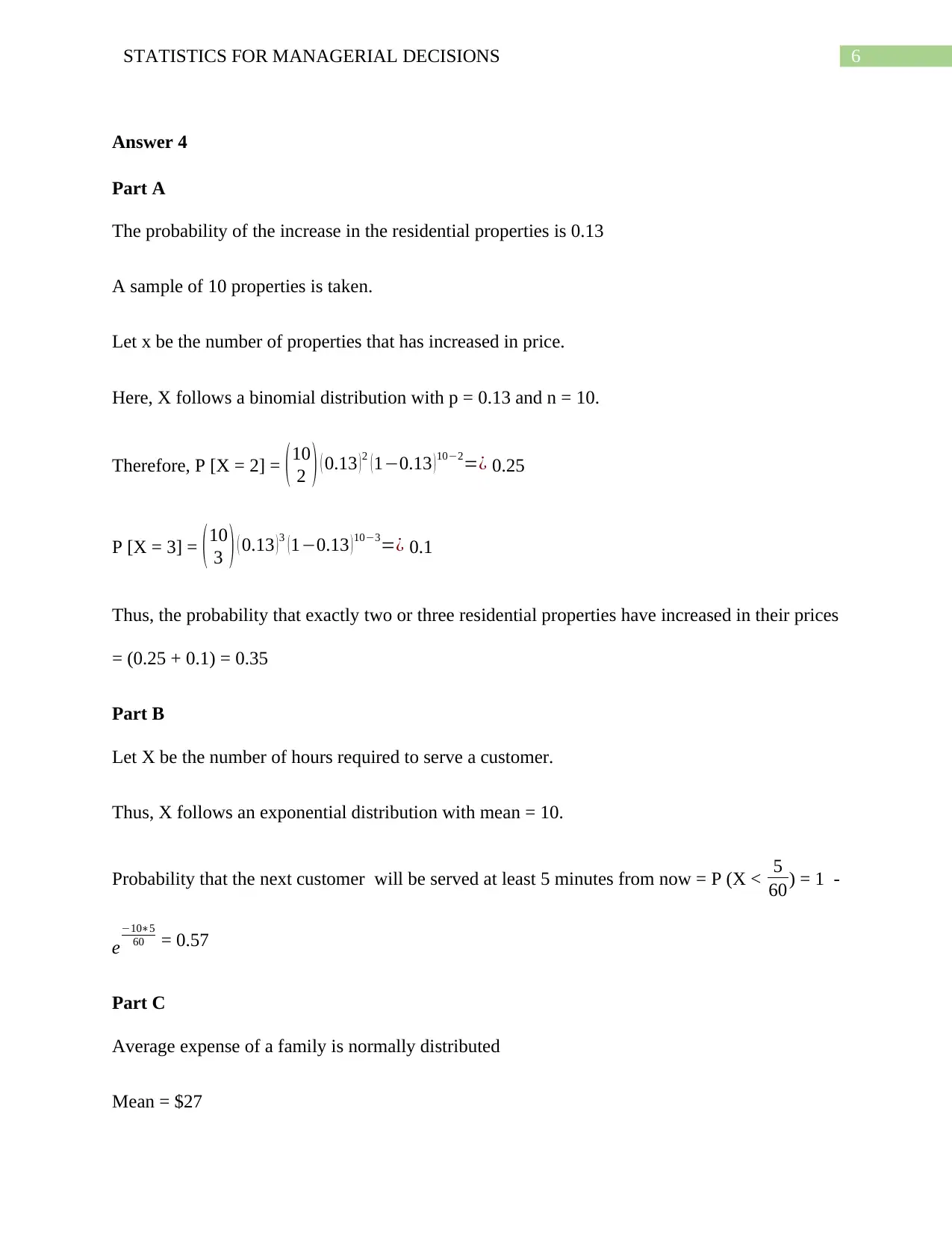
Answer 4
Part A
The probability of the increase in the residential properties is 0.13
A sample of 10 properties is taken.
Let x be the number of properties that has increased in price.
Here, X follows a binomial distribution with p = 0.13 and n = 10.
Therefore, P [X = 2] = ( 10
2 ) ( 0.13 ) 2 ( 1−0.13 ) 10−2=¿ 0.25
P [X = 3] = ( 10
3 ) ( 0.13 ) 3 ( 1−0.13 ) 10−3=¿ 0.1
Thus, the probability that exactly two or three residential properties have increased in their prices
= (0.25 + 0.1) = 0.35
Part B
Let X be the number of hours required to serve a customer.
Thus, X follows an exponential distribution with mean = 10.
Probability that the next customer will be served at least 5 minutes from now = P (X < 5
60) = 1 -
e
−10∗5
60 = 0.57
Part C
Average expense of a family is normally distributed
Mean = $27

7STATISTICS FOR MANAGERIAL DECISIONS
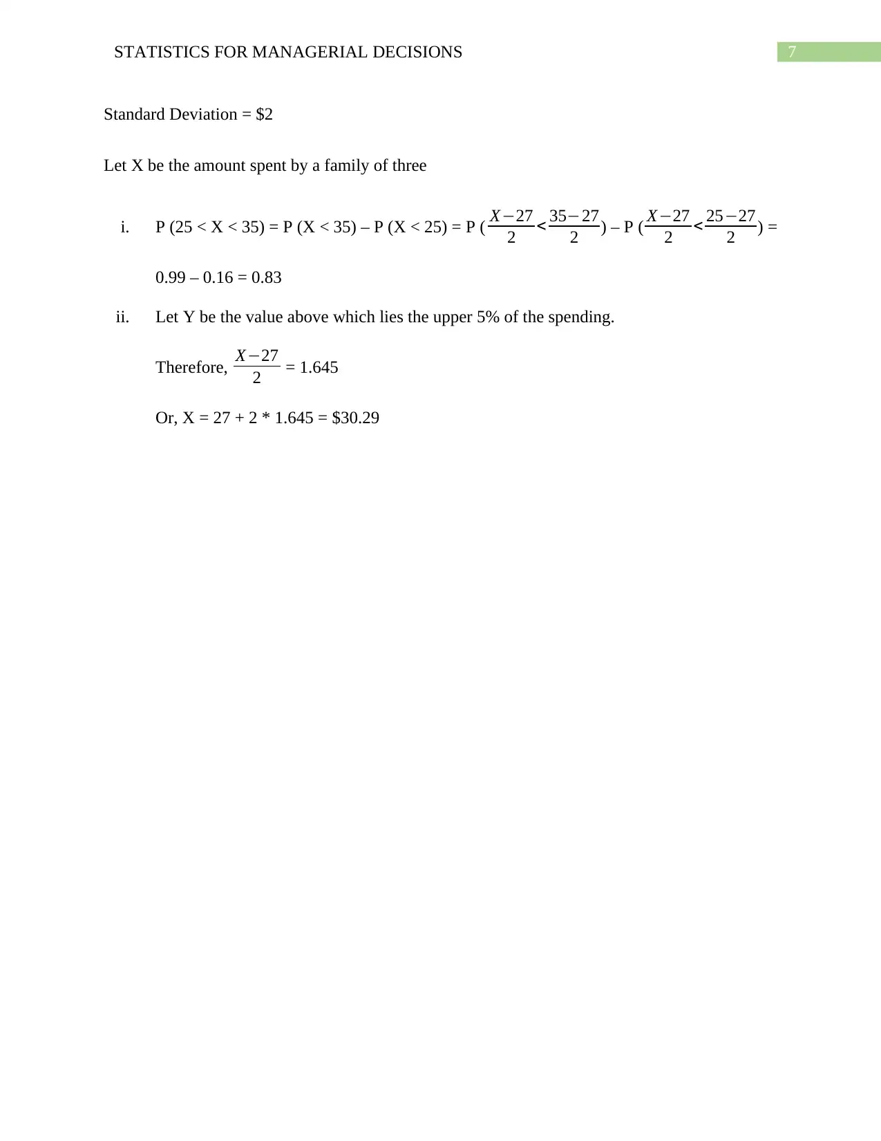
Standard Deviation = $2
Let X be the amount spent by a family of three
i. P (25 < X < 35) = P (X < 35) – P (X < 25) = P ( X−27
2 < 35−27
2 ) – P ( X−27
2 < 25−27
2 ) =
0.99 – 0.16 = 0.83
ii. Let Y be the value above which lies the upper 5% of the spending.
Therefore, X−27
2 = 1.645
Or, X = 27 + 2 * 1.645 = $30.29

8STATISTICS FOR MANAGERIAL DECISIONS
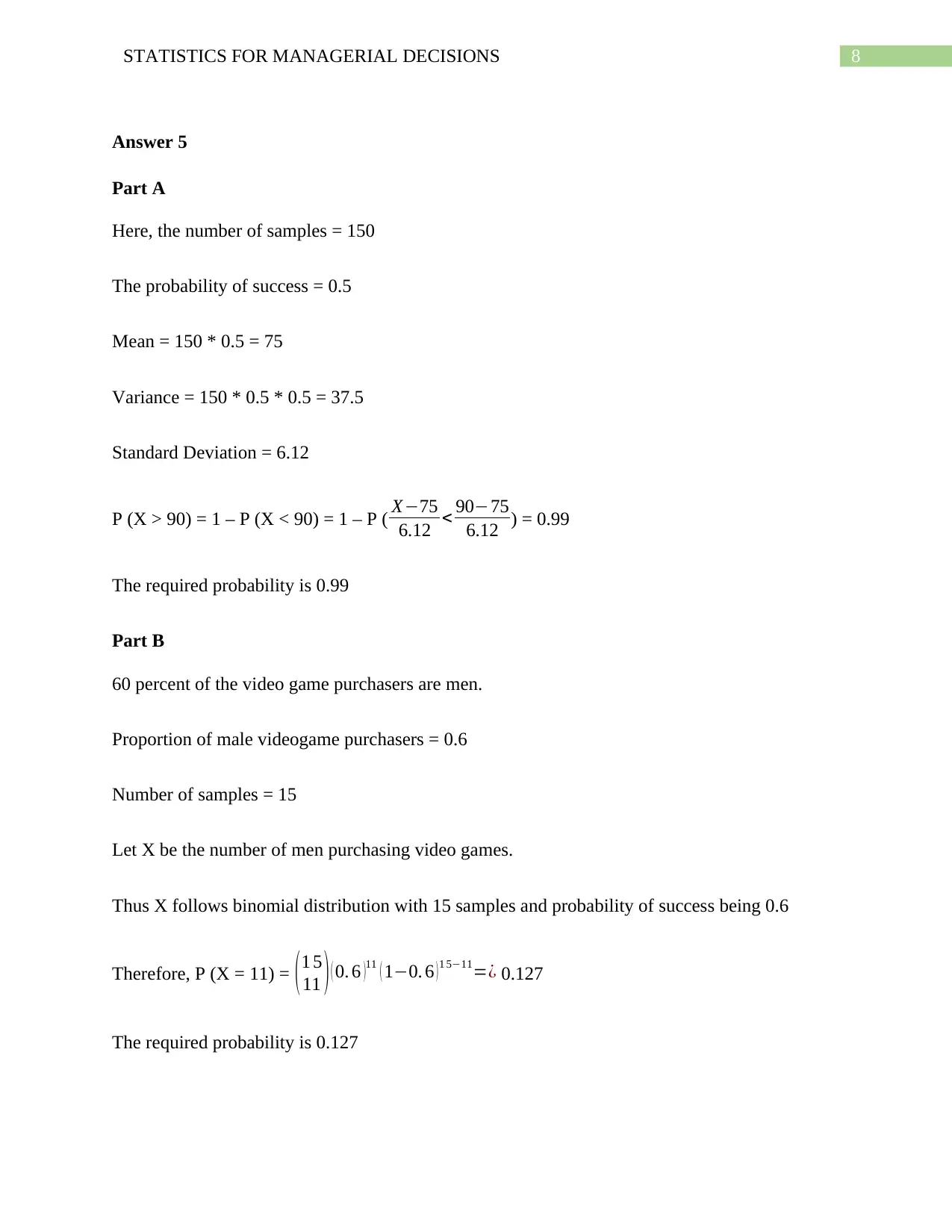
Answer 5
Part A
Here, the number of samples = 150
The probability of success = 0.5
Mean = 150 * 0.5 = 75
Variance = 150 * 0.5 * 0.5 = 37.5
Standard Deviation = 6.12
P (X > 90) = 1 – P (X < 90) = 1 – P ( X−75
6.12 < 90−75
6.12 ) = 0.99
The required probability is 0.99
Part B
60 percent of the video game purchasers are men.
Proportion of male videogame purchasers = 0.6
Number of samples = 15
Let X be the number of men purchasing video games.
Thus X follows binomial distribution with 15 samples and probability of success being 0.6
Therefore, P (X = 11) = ( 1 5
11 ) ( 0. 6 )11 ( 1−0. 6 ) 1 5−11=¿ 0.127
The required probability is 0.127

9STATISTICS FOR MANAGERIAL DECISIONS
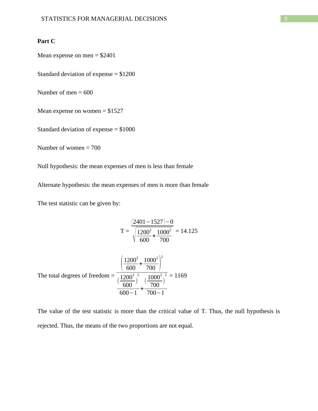
Part C
Mean expense on men = $2401
Standard deviation of expense = $1200
Number of men = 600
Mean expense on women = $1527
Standard deviation of expense = $1000
Number of women = 700
Null hypothesis: the mean expenses of men is less than female
Alternate hypothesis: the mean expenses of men is more than female
The test statistic can be given by:
T =
( 2401−1527 ) −0
√ 12002
600 + 10002
700
= 14.125
The total degrees of freedom =
( 12002
600 + 10002
700 )2
( 12002
600 )
2
600−1 +
( 10002
700 )
2
700−1
= 1169
The value of the test statistic is more than the critical value of T. Thus, the null hypothesis is
rejected. Thus, the means of the two proportions are not equal.