Statistics for Managerial Decisions with solved assignments and graphs

Get solved assignments and essays on Statistics for Managerial Decisions. Learn about probability, Poisson distribution, normal distribution, and more. Access graphs and charts for better understanding.

STATISTICS FOR MANAGERIAL DECISIONS
STUDENT ID:
[Pick the date]

Question 1
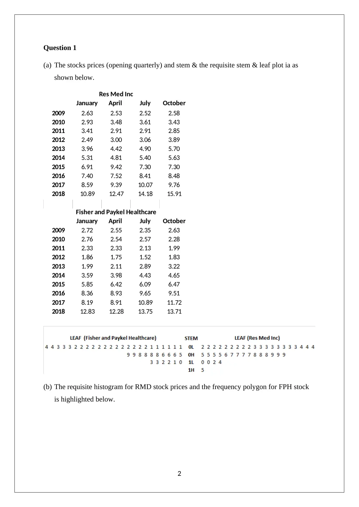
(a) The stocks prices (opening quarterly) and stem & the requisite stem & leaf plot ia as
shown below.
January April July October
2009 2.63 2.53 2.52 2.58
2010 2.93 3.48 3.61 3.43
2011 3.41 2.91 2.91 2.85
2012 2.49 3.00 3.06 3.89
2013 3.96 4.42 4.90 5.70
2014 5.31 4.81 5.40 5.63
2015 6.91 9.42 7.30 7.30
2016 7.40 7.52 8.41 8.48
2017 8.59 9.39 10.07 9.76
2018 10.89 12.47 14.18 15.91
January April July October
2009 2.72 2.55 2.35 2.63
2010 2.76 2.54 2.57 2.28
2011 2.33 2.33 2.13 1.99
2012 1.86 1.75 1.52 1.83
2013 1.99 2.11 2.89 3.22
2014 3.59 3.98 4.43 4.65
2015 5.85 6.42 6.09 6.47
2016 8.36 8.93 9.65 9.51
2017 8.19 8.91 10.89 11.72
2018 12.83 12.28 13.75 13.71
Res Med Inc
Fisher and Paykel Healthcare
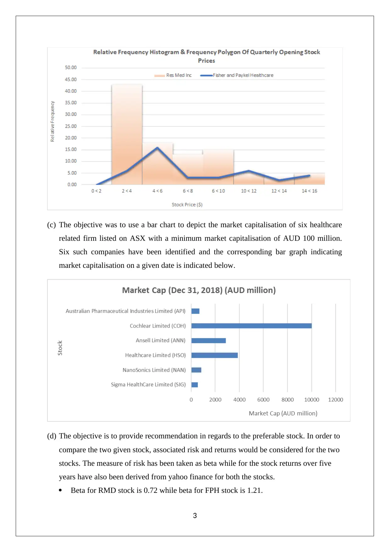
(b) The requisite histogram for RMD stock prices and the frequency polygon for FPH stock
is highlighted below.
2

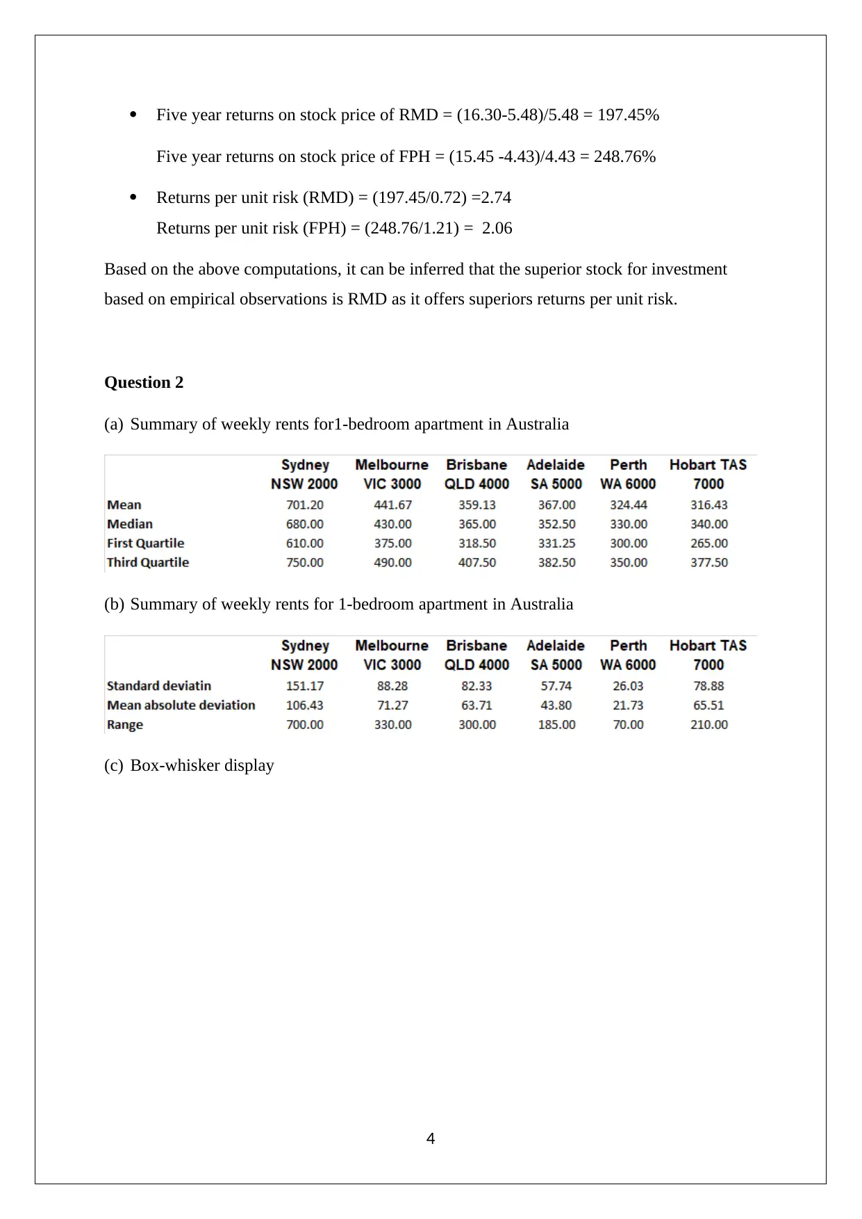
(c) The objective was to use a bar chart to depict the market capitalisation of six healthcare
related firm listed on ASX with a minimum market capitalisation of AUD 100 million.
Six such companies have been identified and the corresponding bar graph indicating
market capitalisation on a given date is indicated below.
(d) The objective is to provide recommendation in regards to the preferable stock. In order to
compare the two given stock, associated risk and returns would be considered for the two
stocks. The measure of risk has been taken as beta while for the stock returns over five
years have also been derived from yahoo finance for both the stocks.
 Beta for RMD stock is 0.72 while beta for FPH stock is 1.21.
3

 Five year returns on stock price of RMD = (16.30-5.48)/5.48 = 197.45%
Five year returns on stock price of FPH = (15.45 -4.43)/4.43 = 248.76%
 Returns per unit risk (RMD) = (197.45/0.72) =2.74
Returns per unit risk (FPH) = (248.76/1.21) = 2.06
Based on the above computations, it can be inferred that the superior stock for investment
based on empirical observations is RMD as it offers superiors returns per unit risk.
Question 2
(a) Summary of weekly rents for1-bedroom apartment in Australia
(b) Summary of weekly rents for 1-bedroom apartment in Australia
(c) Box-whisker display
4

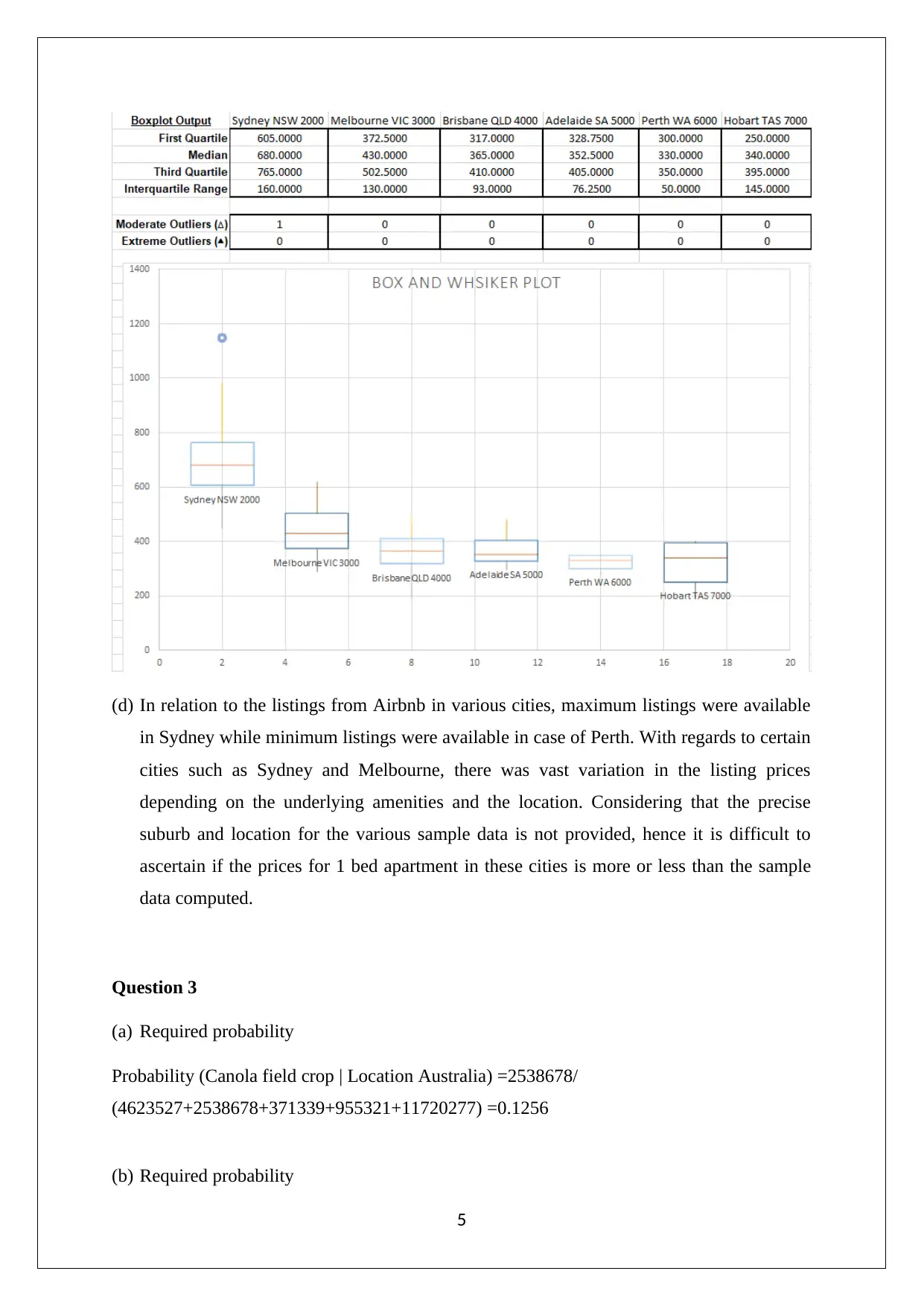
(d) In relation to the listings from Airbnb in various cities, maximum listings were available
in Sydney while minimum listings were available in case of Perth. With regards to certain
cities such as Sydney and Melbourne, there was vast variation in the listing prices
depending on the underlying amenities and the location. Considering that the precise
suburb and location for the various sample data is not provided, hence it is difficult to
ascertain if the prices for 1 bed apartment in these cities is more or less than the sample
data computed.
Question 3
(a) Required probability
Probability (Canola field crop | Location Australia) =2538678/
(4623527+2538678+371339+955321+11720277) =0.1256
(b) Required probability
5

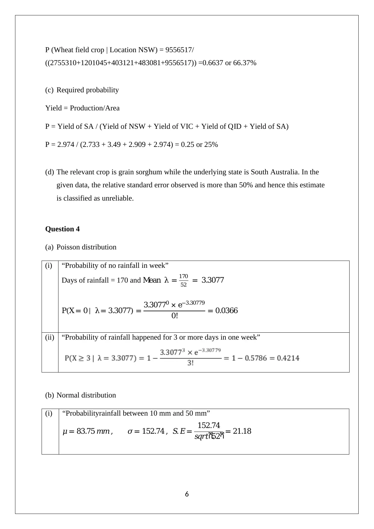
P (Wheat field crop | Location NSW) = 9556517/
((2755310+1201045+403121+483081+9556517)) =0.6637 or 66.37%
(c) Required probability
P = Yield of SA / (Yield of NSW + Yield of VIC + Yield of QID + Yield of SA)
P = 2.974 / (2.733 + 3.49 + 2.909 + 2.974) = 0.25 or 25%
Yield = Production/Area
(d) The relevant crop is grain sorghum while the underlying state is South Australia. In the
given data, the relative standard error observed is more than 50% and hence this estimate
is classified as unreliable.
Question 4
(a) Poisson distribution
(i) “Probability of no rainfall in week”
Days of rainfall = 170 and Mean λ = 170
52 = 3.3077
P(X = 0 | λ= 3.3077) = 3.30770 × e−3.30779
0! = 0.0366
(ii) “Probability of rainfall happened for 3 or more days in one week”
(b) Normal distribution
(i) “Probabilityrainfall between 10 mm and 50 mm”
𝜇 = 83.75 𝑚𝑚 , 𝜎= 152.74 , 𝑆.𝐸= 152.74
𝑠𝑞𝑟𝑡ሺ52ሻ= 21.18
6

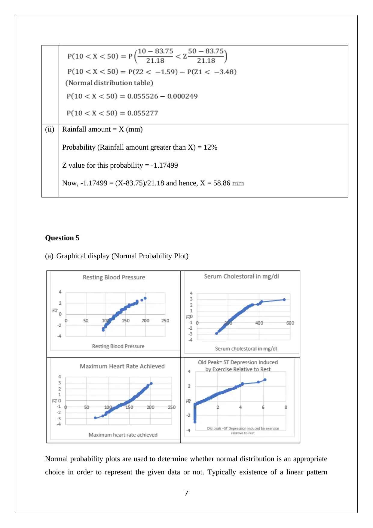
(ii) Rainfall amount = X (mm)
Probability (Rainfall amount greater than X) = 12%
Z value for this probability = -1.17499
Now, -1.17499 = (X-83.75)/21.18 and hence, X = 58.86 mm
Question 5
(a) Graphical display (Normal Probability Plot)
Normal probability plots are used to determine whether normal distribution is an appropriate
choice in order to represent the given data or not. Typically existence of a linear pattern
7

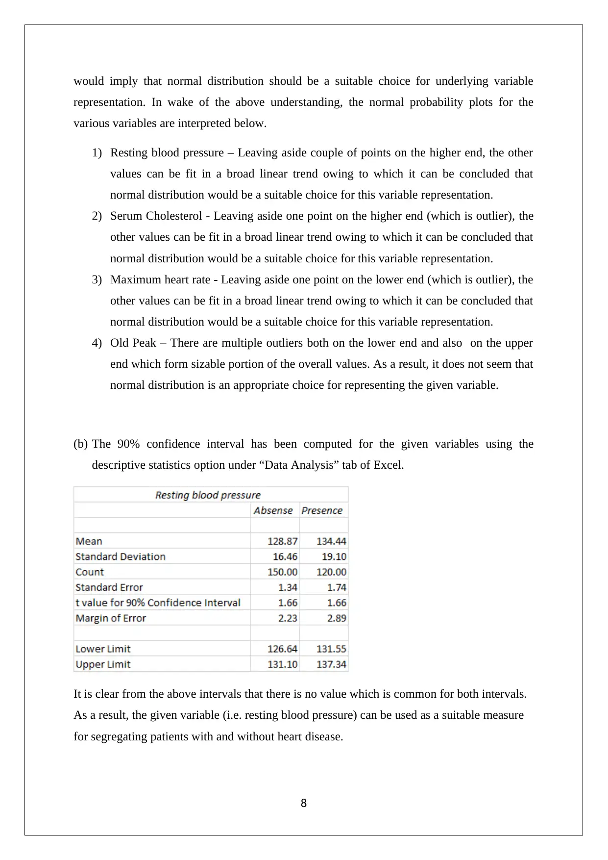
would imply that normal distribution should be a suitable choice for underlying variable
representation. In wake of the above understanding, the normal probability plots for the
various variables are interpreted below.
1) Resting blood pressure – Leaving aside couple of points on the higher end, the other
values can be fit in a broad linear trend owing to which it can be concluded that
normal distribution would be a suitable choice for this variable representation.
2) Serum Cholesterol - Leaving aside one point on the higher end (which is outlier), the
other values can be fit in a broad linear trend owing to which it can be concluded that
normal distribution would be a suitable choice for this variable representation.
3) Maximum heart rate - Leaving aside one point on the lower end (which is outlier), the
other values can be fit in a broad linear trend owing to which it can be concluded that
normal distribution would be a suitable choice for this variable representation.
4) Old Peak – There are multiple outliers both on the lower end and also on the upper
end which form sizable portion of the overall values. As a result, it does not seem that
normal distribution is an appropriate choice for representing the given variable.
(b) The 90% confidence interval has been computed for the given variables using the
descriptive statistics option under “Data Analysis” tab of Excel.
It is clear from the above intervals that there is no value which is common for both intervals.
As a result, the given variable (i.e. resting blood pressure) can be used as a suitable measure
for segregating patients with and without heart disease.
8

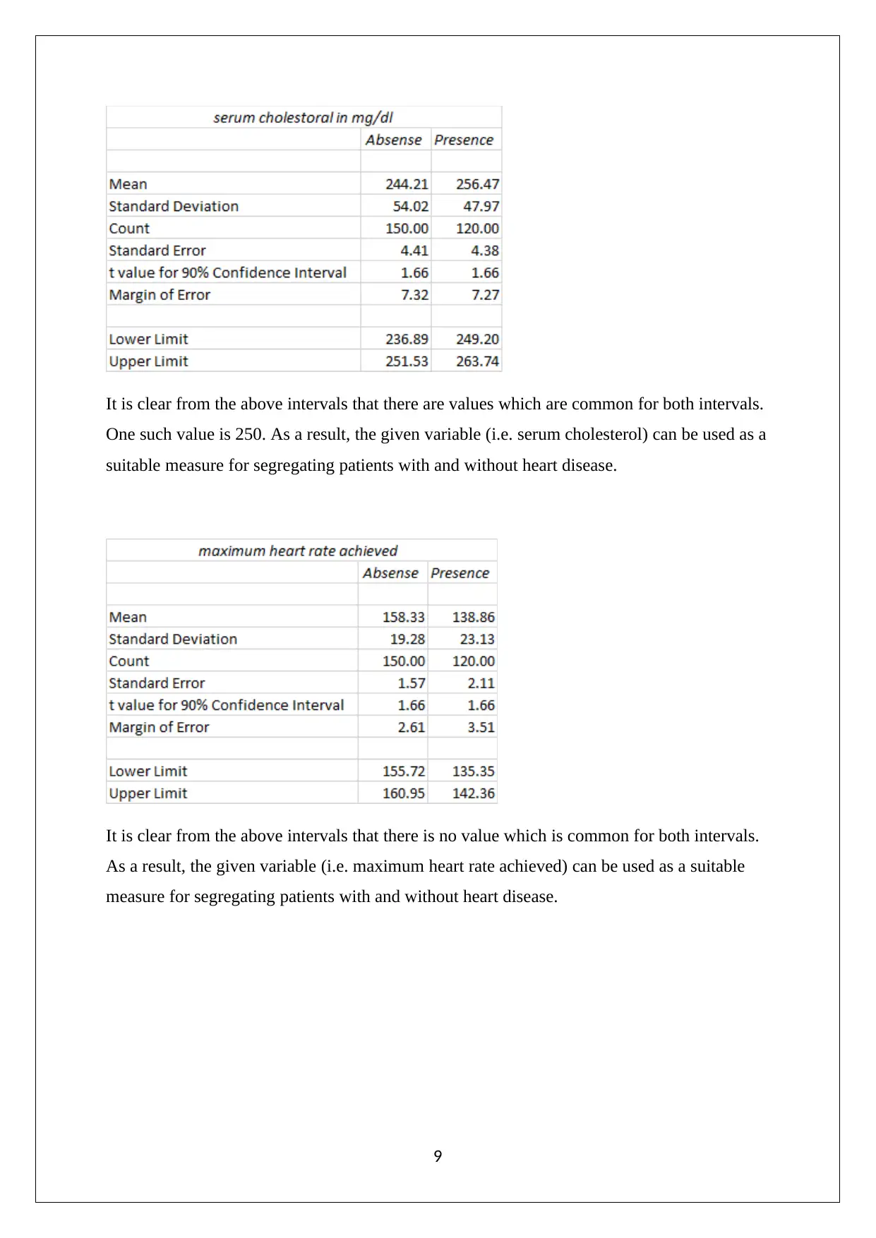
It is clear from the above intervals that there are values which are common for both intervals.
One such value is 250. As a result, the given variable (i.e. serum cholesterol) can be used as a
suitable measure for segregating patients with and without heart disease.
It is clear from the above intervals that there is no value which is common for both intervals.
As a result, the given variable (i.e. maximum heart rate achieved) can be used as a suitable
measure for segregating patients with and without heart disease.
9

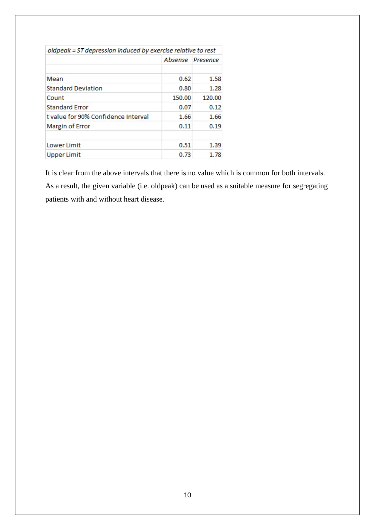
It is clear from the above intervals that there is no value which is common for both intervals.
As a result, the given variable (i.e. oldpeak) can be used as a suitable measure for segregating
patients with and without heart disease.
10