Statistics: Analysis of Gender Gap in Salary

This article provides an analysis of the gender gap in salary using descriptive and inferential statistics. The data set is collected from the Australian Taxation Office (ATO) and a ground survey. The article includes tables, charts, and hypothesis testing to draw conclusions about the gender gap in salary.

Running head: STATISTICS
Statistics
Name of the Student:
Name of the University:
Author’s Note:

1STATISTICS
Table of Contents
Section 1: Introduction:..............................................................................................................2
Answer 1.a)............................................................................................................................2
Answer 1. b)...........................................................................................................................2
Answer 1. c)...........................................................................................................................2
Section 2: Descriptive Statistics.................................................................................................3
Answer 2. a)...........................................................................................................................3
Answer 2. b)...........................................................................................................................3
Answer 2. c)...........................................................................................................................4
Answer 2. d)...........................................................................................................................4
Section 3: Inferential Statistics...................................................................................................5
Answer 3.a)............................................................................................................................5
Answer 3.b)............................................................................................................................6
Answer 3. c)...........................................................................................................................7
Answer 3. d)...........................................................................................................................8
Section 4: Discussion and Conclusion.......................................................................................9
Answer 4. a)...........................................................................................................................9
Answer 4. b)...........................................................................................................................9
References:...............................................................................................................................11

2STATISTICS
Section 1: Introduction:
Answer 1.a)
The data set is collected from the Australian Taxation Office (ATO). The data set
would help to find the gender gap of salary between men and women. The reasons of gender
gap generate the discrimination of hiring in the job. The salary as well as occupation
according to the different gender varies significantly. The data set summarises the analysis
regarding job profile of women and men in different industries. Their salary or wage and
donation or gift amounts. We considered the data file as “College data”. The data set includes
totally 1000 samples.
The research question is:
“Is there any difference of the average salary amount between male and females in data
set2?” (Dietl et al. 2012).
Answer 1. b)
The data set 1 is a secondary data. The data is not collected by researcher himself.
ATO has delivered the data to the researcher for analysis.
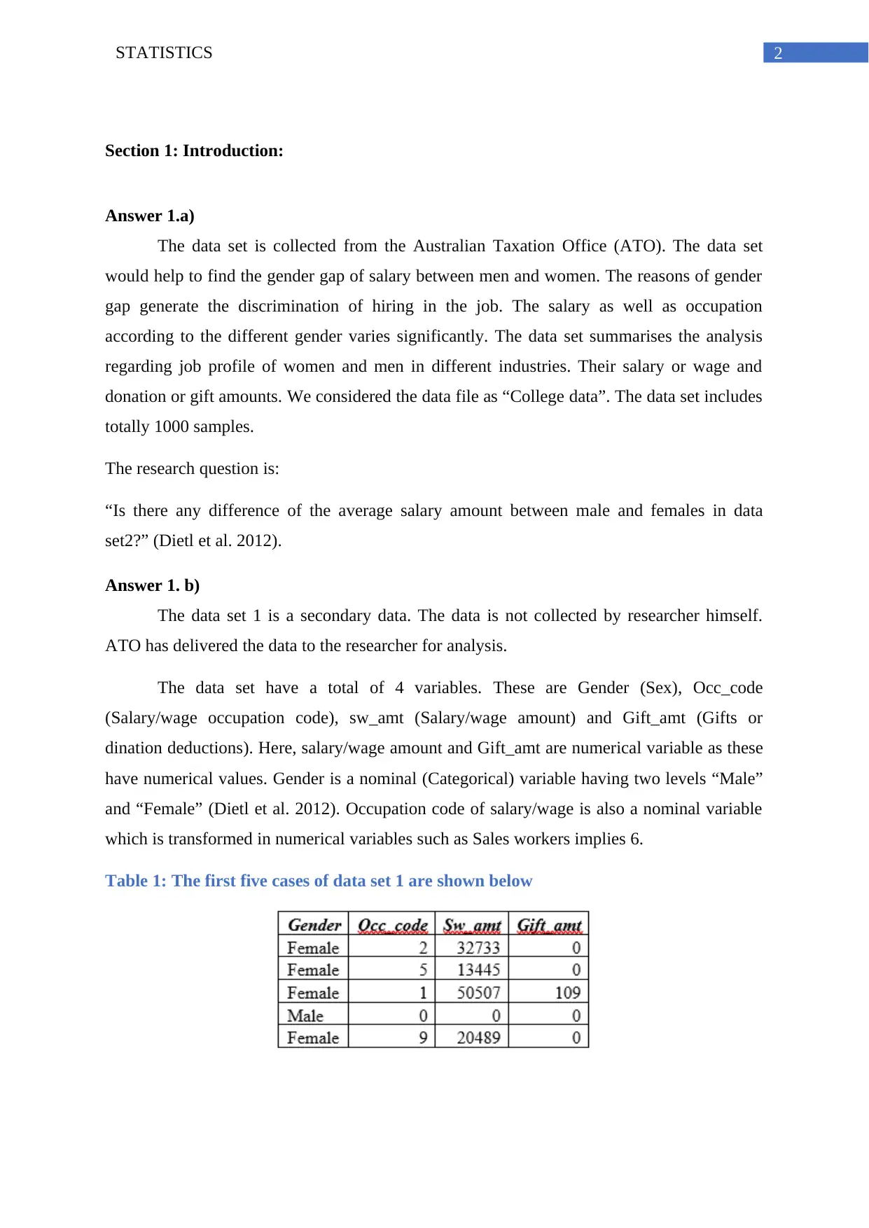
The data set have a total of 4 variables. These are Gender (Sex), Occ_code
(Salary/wage occupation code), sw_amt (Salary/wage amount) and Gift_amt (Gifts or
dination deductions). Here, salary/wage amount and Gift_amt are numerical variable as these
have numerical values. Gender is a nominal (Categorical) variable having two levels “Male”
and “Female” (Dietl et al. 2012). Occupation code of salary/wage is also a nominal variable
which is transformed in numerical variables such as Sales workers implies 6.
Table 1: The first five cases of data set 1 are shown below

3STATISTICS
Answer 1. c)
Not only that, in the second part, the data of only gender type and salary/wage is
tabulated with the help of survey. This second data set is named as “College” data. The data
is collected by random sampling method. The simple data collection method randomly had
received the responses from 100 males and females of the college. Out of them, only 63
people, responded about their amount of salary.
The data set is collected with the help of ground survey with a simple questionnaire of
two questions: 1) “What is your gender?” 2) “What is your salary amount?”.
The data is primary in nature to the researcher. The data set involves one numerical
(salary/wage) and one categorical (Gender) variable.
Section 2: Descriptive Statistics
Answer 2. a)
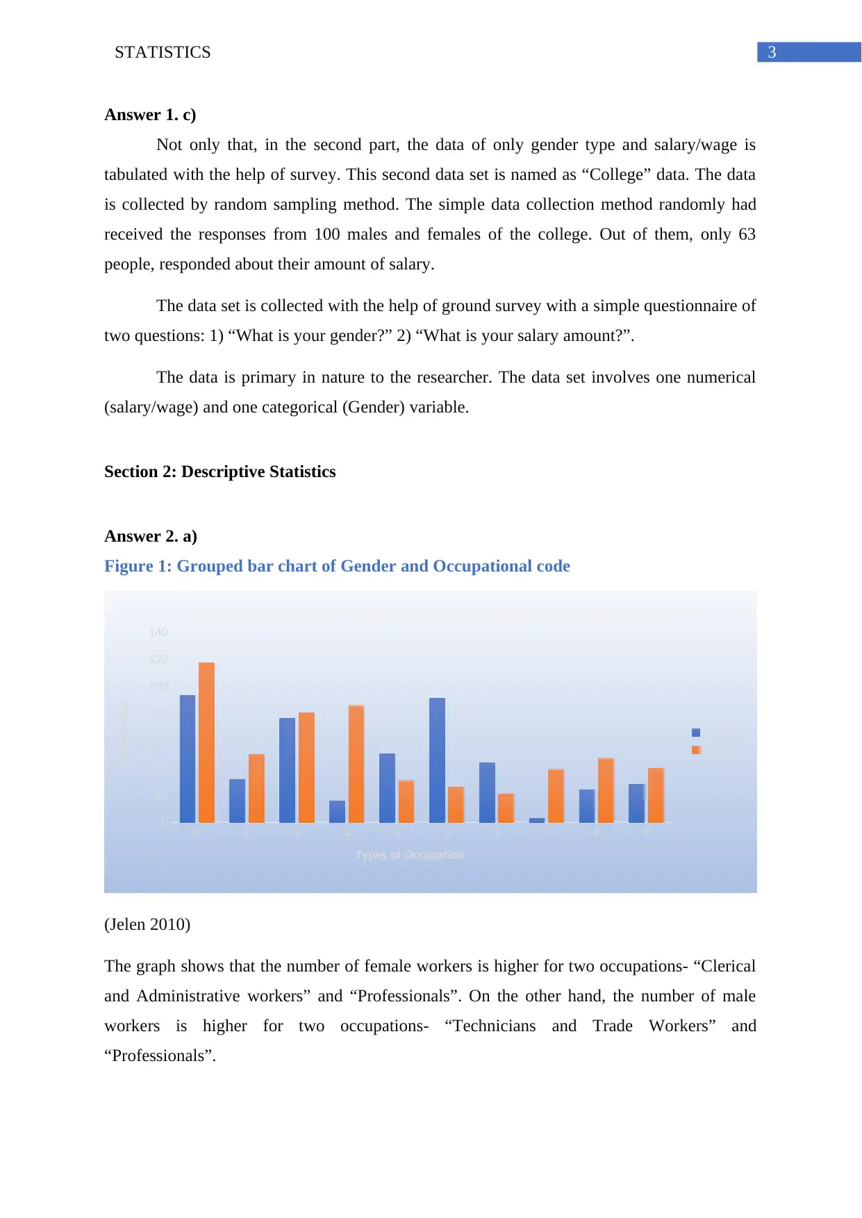
Figure 1: Grouped bar chart of Gender and Occupational code
0 1 2 3 4 5 6 7 8 9
0
20
40
60
80
100
120
140
Fre que ncie s of type s of occupati on ge nde r wise
Female
Male
Types of Occupation
Frequencies
(Jelen 2010)
The graph shows that the number of female workers is higher for two occupations- “Clerical
and Administrative workers” and “Professionals”. On the other hand, the number of male
workers is higher for two occupations- “Technicians and Trade Workers” and
“Professionals”.

4STATISTICS
Answer 2. b)
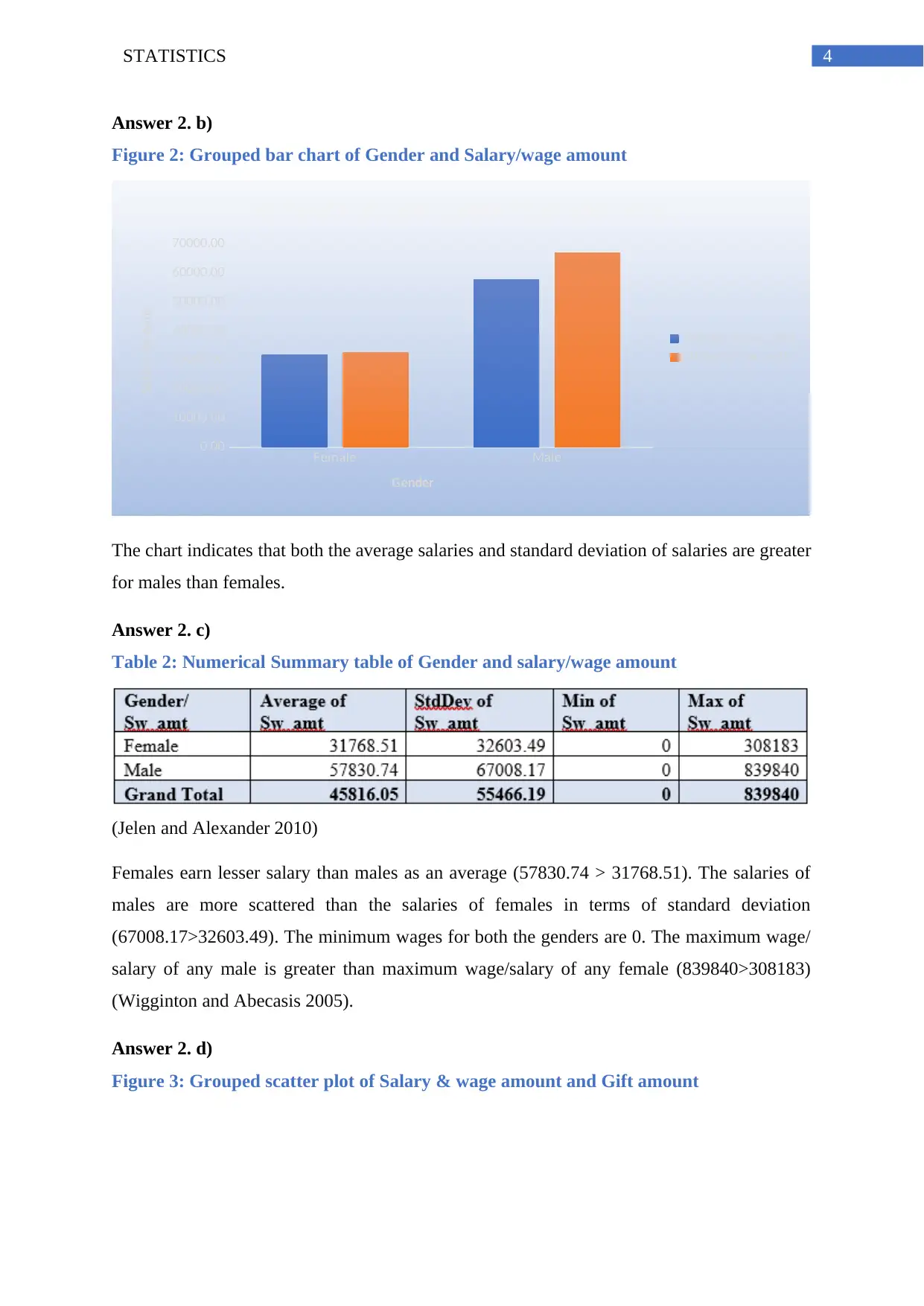
Figure 2: Grouped bar chart of Gender and Salary/wage amount
Female Male
0.00
10000.00
20000.00
30000.00
40000.00
50000.00
60000.00
70000.00
Summary of salary amount ge nde r wise
Average of Sw_amt
StdDev of Sw_amt
Gender
Salary Amount
The chart indicates that both the average salaries and standard deviation of salaries are greater
for males than females.
Answer 2. c)
Table 2: Numerical Summary table of Gender and salary/wage amount
(Jelen and Alexander 2010)
Females earn lesser salary than males as an average (57830.74 > 31768.51). The salaries of
males are more scattered than the salaries of females in terms of standard deviation
(67008.17>32603.49). The minimum wages for both the genders are 0. The maximum wage/
salary of any male is greater than maximum wage/salary of any female (839840>308183)
(Wigginton and Abecasis 2005).
Answer 2. d)
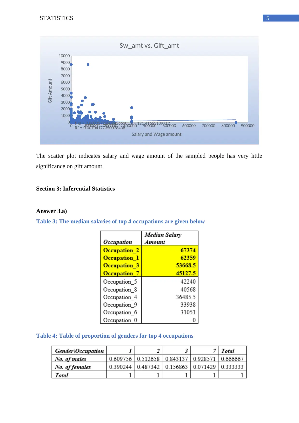
Figure 3: Grouped scatter plot of Salary & wage amount and Gift amount

5STATISTICS
0 100000 200000 300000 400000 500000 600000 700000 800000 900000
0
1000
2000
3000
4000
5000
6000
7000
8000
9000
10000
f(x) = 0.000357219094366305 x + 121.41663139712
R² = 0.00104177350078438
Sw_amt vs. Gift_amt
Salary and Wage amount
Gift Amount
The scatter plot indicates salary and wage amount of the sampled people has very little
significance on gift amount.
Section 3: Inferential Statistics
Answer 3.a)
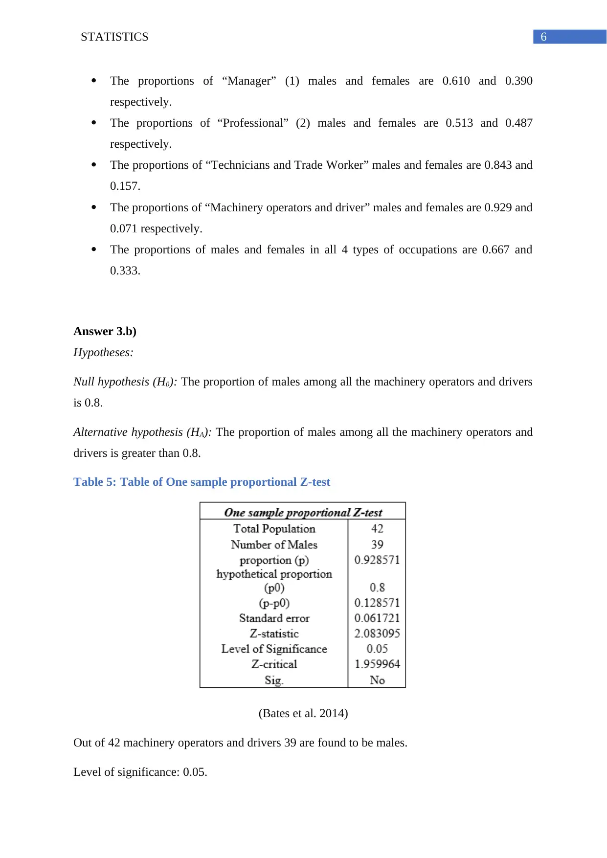
Table 3: The median salaries of top 4 occupations are given below
Table 4: Table of proportion of genders for top 4 occupations

6STATISTICS
 The proportions of “Manager” (1) males and females are 0.610 and 0.390
respectively.
 The proportions of “Professional” (2) males and females are 0.513 and 0.487
respectively.
 The proportions of “Technicians and Trade Worker” males and females are 0.843 and
0.157.
 The proportions of “Machinery operators and driver” males and females are 0.929 and
0.071 respectively.
 The proportions of males and females in all 4 types of occupations are 0.667 and
0.333.
Answer 3.b)
Hypotheses:
Null hypothesis (H0): The proportion of males among all the machinery operators and drivers
is 0.8.
Alternative hypothesis (HA): The proportion of males among all the machinery operators and
drivers is greater than 0.8.
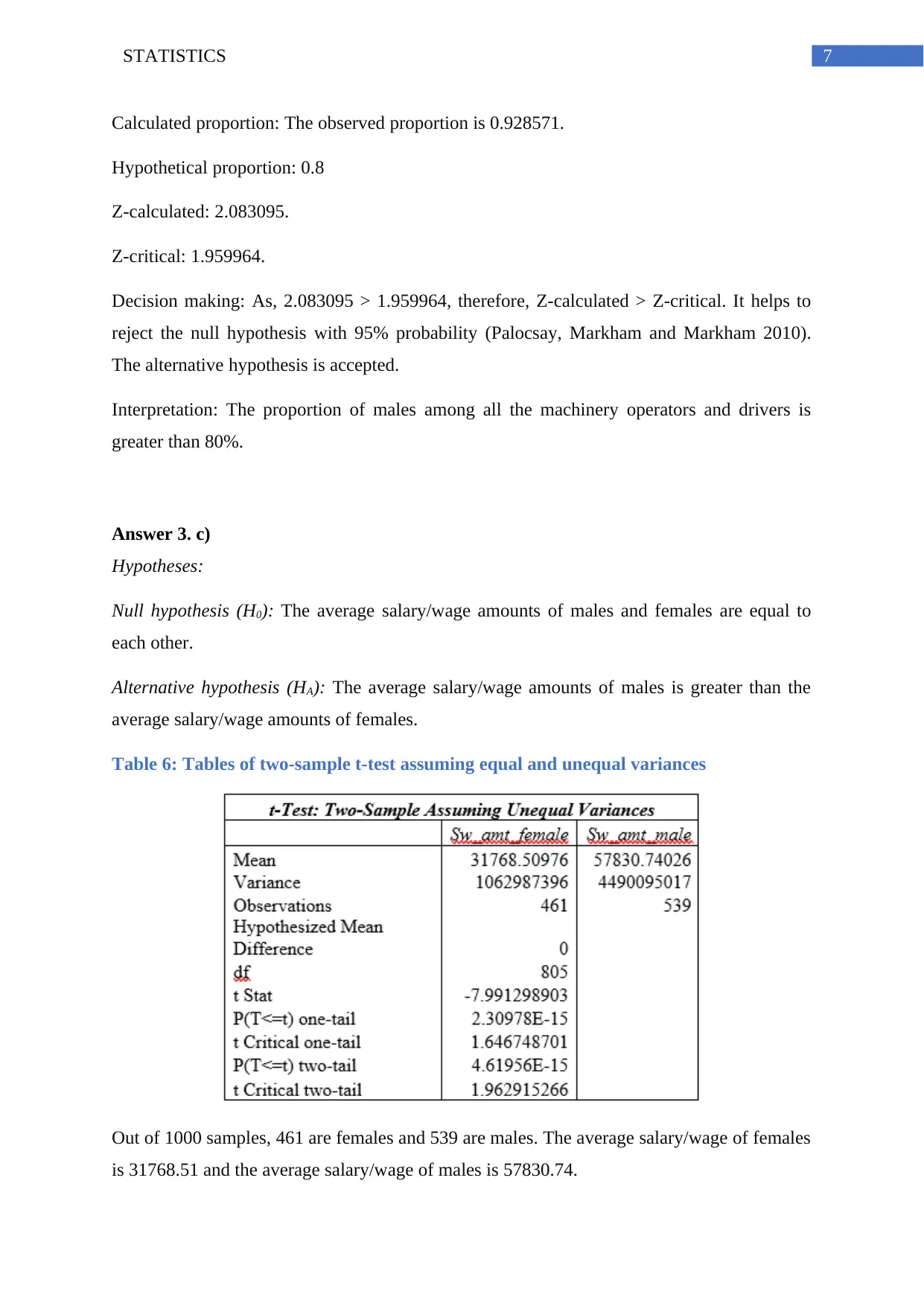
Table 5: Table of One sample proportional Z-test
(Bates et al. 2014)
Out of 42 machinery operators and drivers 39 are found to be males.
Level of significance: 0.05.

7STATISTICS
Calculated proportion: The observed proportion is 0.928571.
Hypothetical proportion: 0.8
Z-calculated: 2.083095.
Z-critical: 1.959964.
Decision making: As, 2.083095 > 1.959964, therefore, Z-calculated > Z-critical. It helps to
reject the null hypothesis with 95% probability (Palocsay, Markham and Markham 2010).
The alternative hypothesis is accepted.
Interpretation: The proportion of males among all the machinery operators and drivers is
greater than 80%.
Answer 3. c)
Hypotheses:
Null hypothesis (H0): The average salary/wage amounts of males and females are equal to
each other.
Alternative hypothesis (HA): The average salary/wage amounts of males is greater than the
average salary/wage amounts of females.
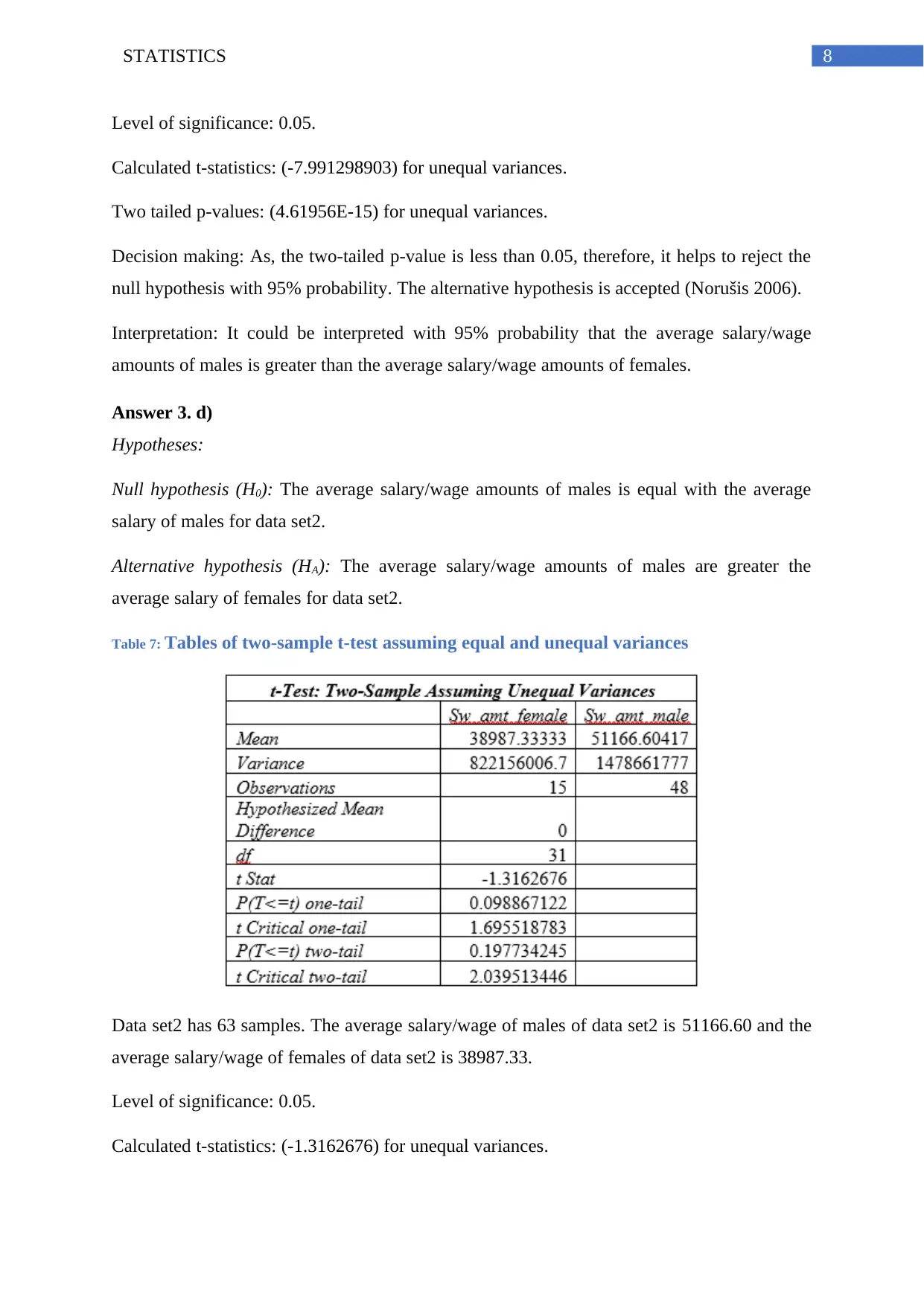
Table 6: Tables of two-sample t-test assuming equal and unequal variances
Out of 1000 samples, 461 are females and 539 are males. The average salary/wage of females
is 31768.51 and the average salary/wage of males is 57830.74.

8STATISTICS
Level of significance: 0.05.
Calculated t-statistics: (-7.991298903) for unequal variances.
Two tailed p-values: (4.61956E-15) for unequal variances.
Decision making: As, the two-tailed p-value is less than 0.05, therefore, it helps to reject the
null hypothesis with 95% probability. The alternative hypothesis is accepted (Norušis 2006).
Interpretation: It could be interpreted with 95% probability that the average salary/wage
amounts of males is greater than the average salary/wage amounts of females.
Answer 3. d)
Hypotheses:
Null hypothesis (H0): The average salary/wage amounts of males is equal with the average
salary of males for data set2.
Alternative hypothesis (HA): The average salary/wage amounts of males are greater the
average salary of females for data set2.
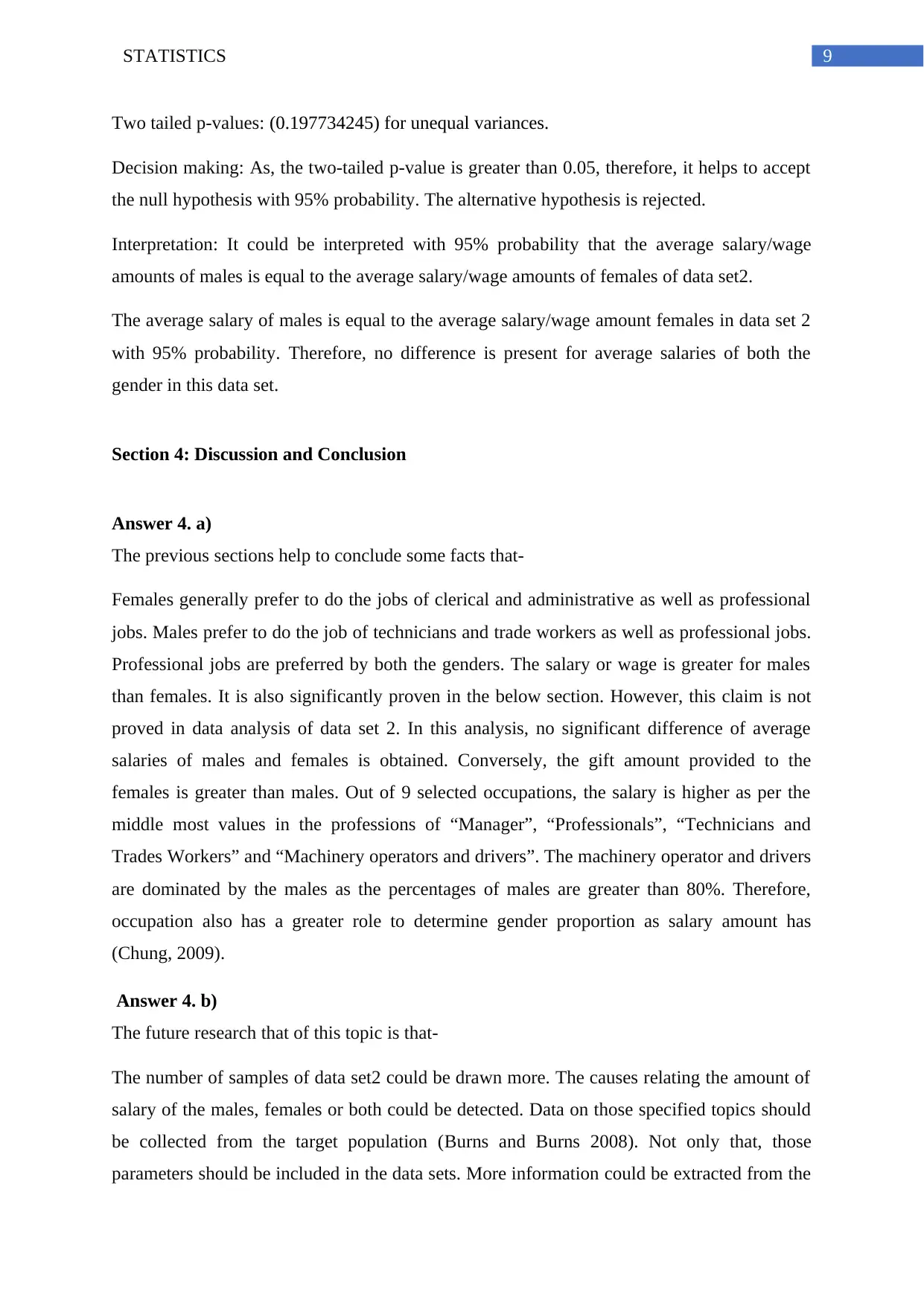
Table 7: Tables of two-sample t-test assuming equal and unequal variances
Data set2 has 63 samples. The average salary/wage of males of data set2 is 51166.60 and the
average salary/wage of females of data set2 is 38987.33.
Level of significance: 0.05.
Calculated t-statistics: (-1.3162676) for unequal variances.

9STATISTICS
Two tailed p-values: (0.197734245) for unequal variances.
Decision making: As, the two-tailed p-value is greater than 0.05, therefore, it helps to accept
the null hypothesis with 95% probability. The alternative hypothesis is rejected.
Interpretation: It could be interpreted with 95% probability that the average salary/wage
amounts of males is equal to the average salary/wage amounts of females of data set2.
The average salary of males is equal to the average salary/wage amount females in data set 2
with 95% probability. Therefore, no difference is present for average salaries of both the
gender in this data set.
Section 4: Discussion and Conclusion
Answer 4. a)
The previous sections help to conclude some facts that-
Females generally prefer to do the jobs of clerical and administrative as well as professional
jobs. Males prefer to do the job of technicians and trade workers as well as professional jobs.
Professional jobs are preferred by both the genders. The salary or wage is greater for males
than females. It is also significantly proven in the below section. However, this claim is not
proved in data analysis of data set 2. In this analysis, no significant difference of average
salaries of males and females is obtained. Conversely, the gift amount provided to the
females is greater than males. Out of 9 selected occupations, the salary is higher as per the
middle most values in the professions of “Manager”, “Professionals”, “Technicians and
Trades Workers” and “Machinery operators and drivers”. The machinery operator and drivers
are dominated by the males as the percentages of males are greater than 80%. Therefore,
occupation also has a greater role to determine gender proportion as salary amount has
(Chung, 2009).
Answer 4. b)
The future research that of this topic is that-
The number of samples of data set2 could be drawn more. The causes relating the amount of
salary of the males, females or both could be detected. Data on those specified topics should
be collected from the target population (Burns and Burns 2008). Not only that, those
parameters should be included in the data sets. More information could be extracted from the

10STATISTICS
analysed dataset if the information regarding years of experience, educational level, hours of
working and designation of work are added in the data set (Black 2009).
References:
Bates, D., Maechler, M., Bolker, B. and Walker, S., 2014. lme4: Linear mixed-effects models
using Eigen and S4. R package version, 1(7), pp.1-23.
Black, K., 2009. Business statistics: Contemporary decision making. John Wiley & Sons.
Chung, S., Domino, M.E., Stearns, S.C. and Popkin, B.M., 2009. Retirement and physical
activity: analyses by occupation and wealth. American journal of preventive medicine, 36(5),
pp.422-428.
Dietl, H.M., Franck, E., Lang, M. and Rathke, A., 2012. Salary cap regulation in professional
team sports. Contemporary economic policy, 30(3), pp.307-319.
Jelen, B. and Alexander, M., 2010. Pivot Table Data Crunching: Microsoft Excel 2010.
Pearson Education.
Jelen, B., 2010. Charts and Graphs: Microsoft Excel 2010. Que Publishing.
Norušis, M.J., 2006. SPSS 14.0 guide to data analysis. Upper Saddle River, NJ: Prentice
Hall.
Palocsay, S.W., Markham, I.S. and Markham, S.E., 2010. Utilizing and teaching data tools in
Excel for exploratory analysis. Journal of Business Research, 63(2), pp.191-206.
Wigginton, J.E. and Abecasis, G.R., 2005. PEDSTATS: descriptive statistics, graphics and
quality assessment for gene mapping data. Bioinformatics, 21(16), pp.3445-3447.

11STATISTICS