Comprehensive Analysis of Statistical Data: HI6007 Assignment Solution
VerifiedAdded on 2024/05/31
|13
|1872
|264
Homework Assignment
AI Summary
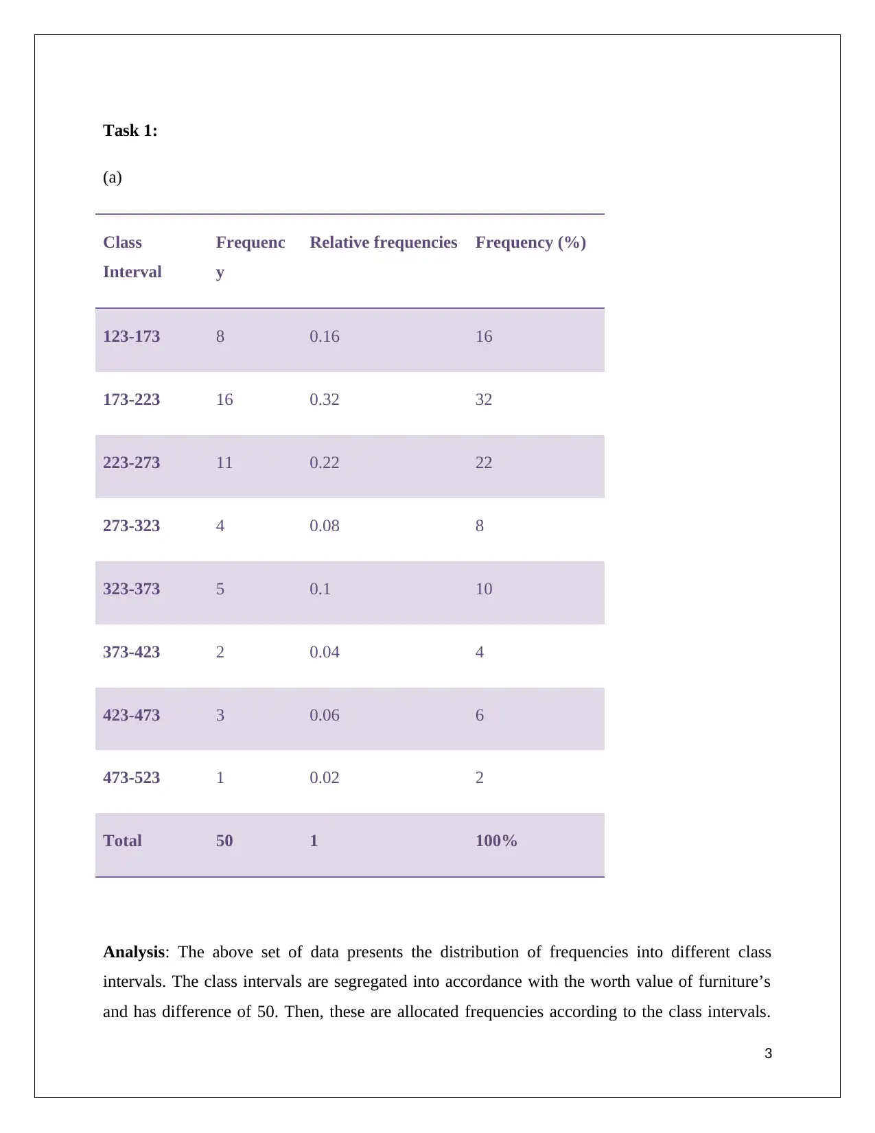
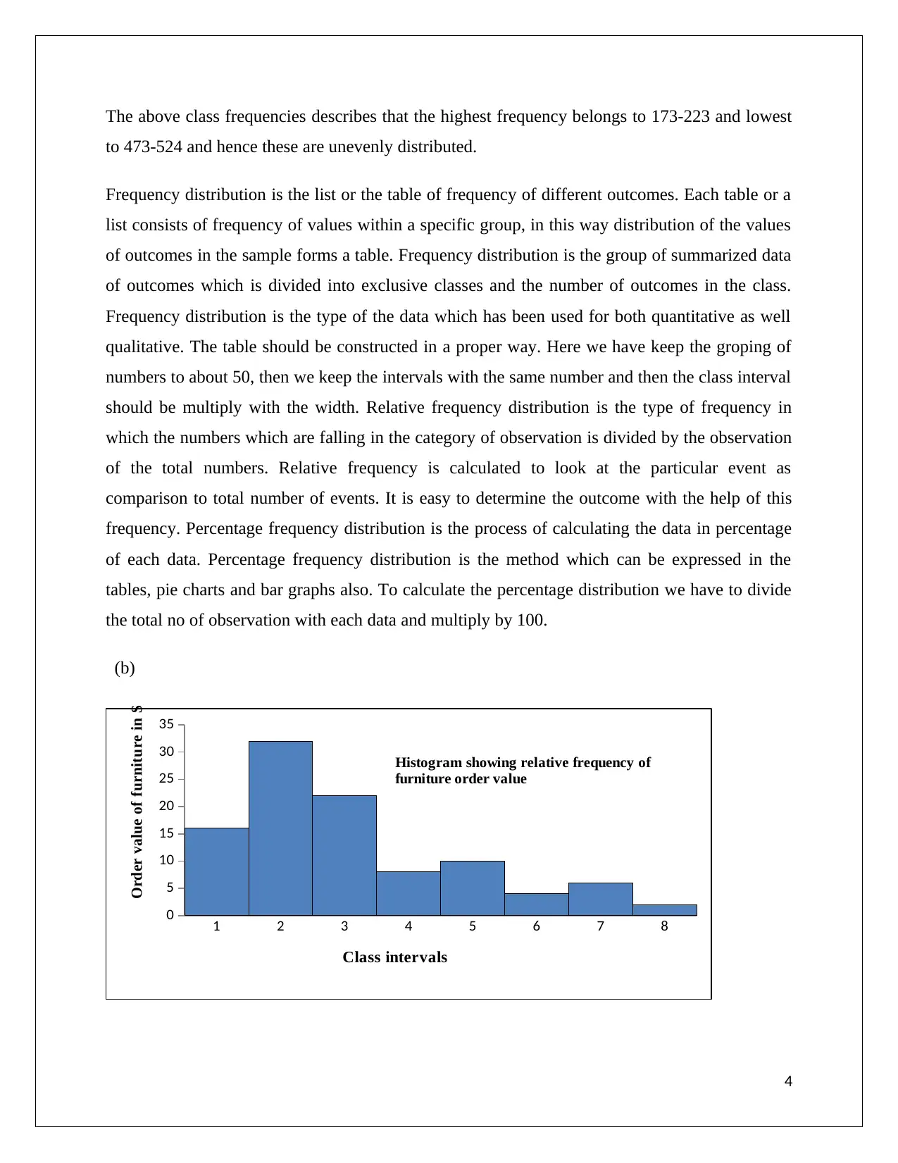
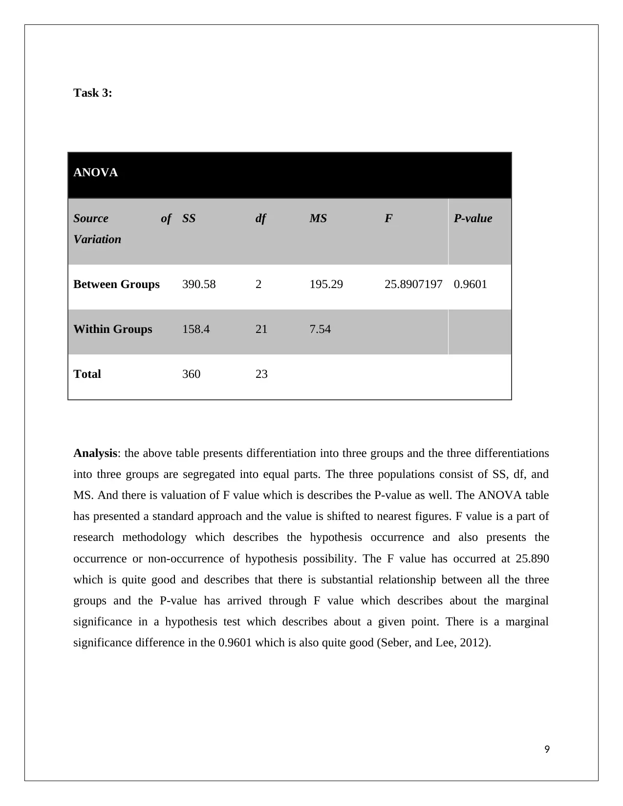
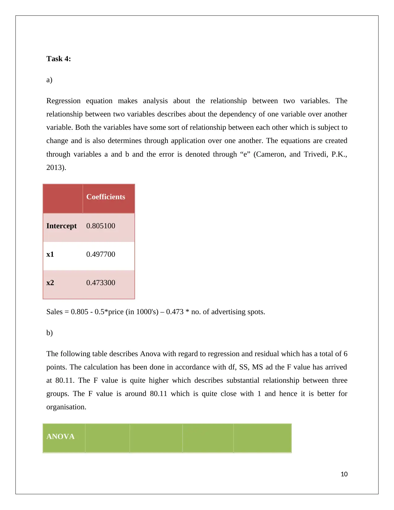
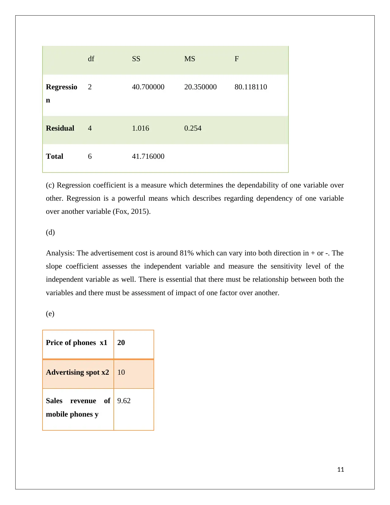
This assignment solution for Statistics HI6007 thoroughly explores frequency distribution, ANOVA, and regression analysis. It begins with constructing frequency tables and histograms to analyze data distribution, followed by an ANOVA table to determine F and P values. The assignment further examines the coefficient of determination and analyzes coefficients, standard errors, and t-statistics. It also covers regression equations, assessing the relationship between variables, and interpreting regression coefficients. Finally, the solution predicts sales revenue based on price and advertising spots, providing a comprehensive overview of statistical concepts and their application. Desklib provides a platform to explore similar solved assignments and past papers.
1 out of 13
Related Documents


Your All-in-One AI-Powered Toolkit for Academic Success.
+13062052269
info@desklib.com
Available 24*7 on WhatsApp / Email
![[object Object]](/_next/static/media/star-bottom.7253800d.svg)
Copyright © 2020–2025 A2Z Services. All Rights Reserved. Developed and managed by ZUCOL.