Statistics HI6007 Group Assignment: Business Start-up Costs and Sales
VerifiedAdded on 2019/10/31
|11
|662
|430
Homework Assignment
AI Summary
This document presents a completed group assignment for the statistics course HI6007. The assignment analyzes business data, focusing on startup costs and annual net sales across different business types. Task 1 involves descriptive statistics (mean, median, mode, range, and standard deviation), frequency and relative frequency distributions, and hypothesis testing using ANOVA to compare the average starting costs of businesses. Task 2 builds a regression model to predict annual net sales based on several independent variables (area, inventory, advertising spend, sales district size, and competitors). The analysis includes the regression equation, R-squared value, ANOVA table, interpretation of slope coefficients, and hypothesis testing for the significance of each variable. The document provides a comprehensive statistical analysis with conclusions drawn from the results.
STATISTICS
HI6007 GROUP ASSIGNMENT
STUDENT ID
[Pick the date]
HI6007 GROUP ASSIGNMENT
STUDENT ID
[Pick the date]
Paraphrase This Document
Need a fresh take? Get an instant paraphrase of this document with our AI Paraphraser
Task 1
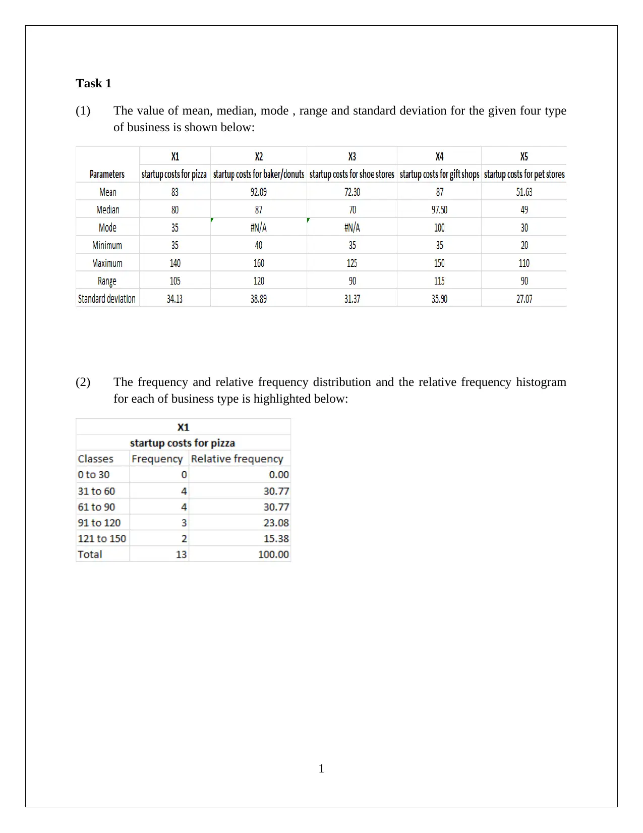
(1) The value of mean, median, mode , range and standard deviation for the given four type
of business is shown below:
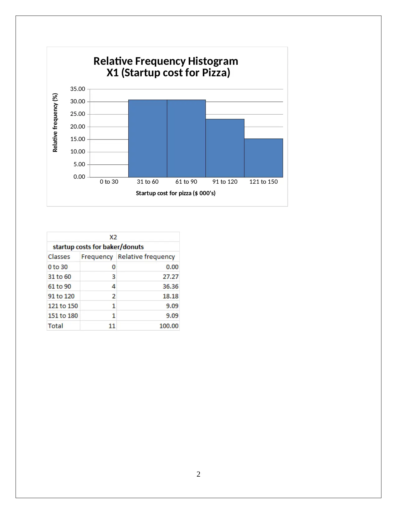
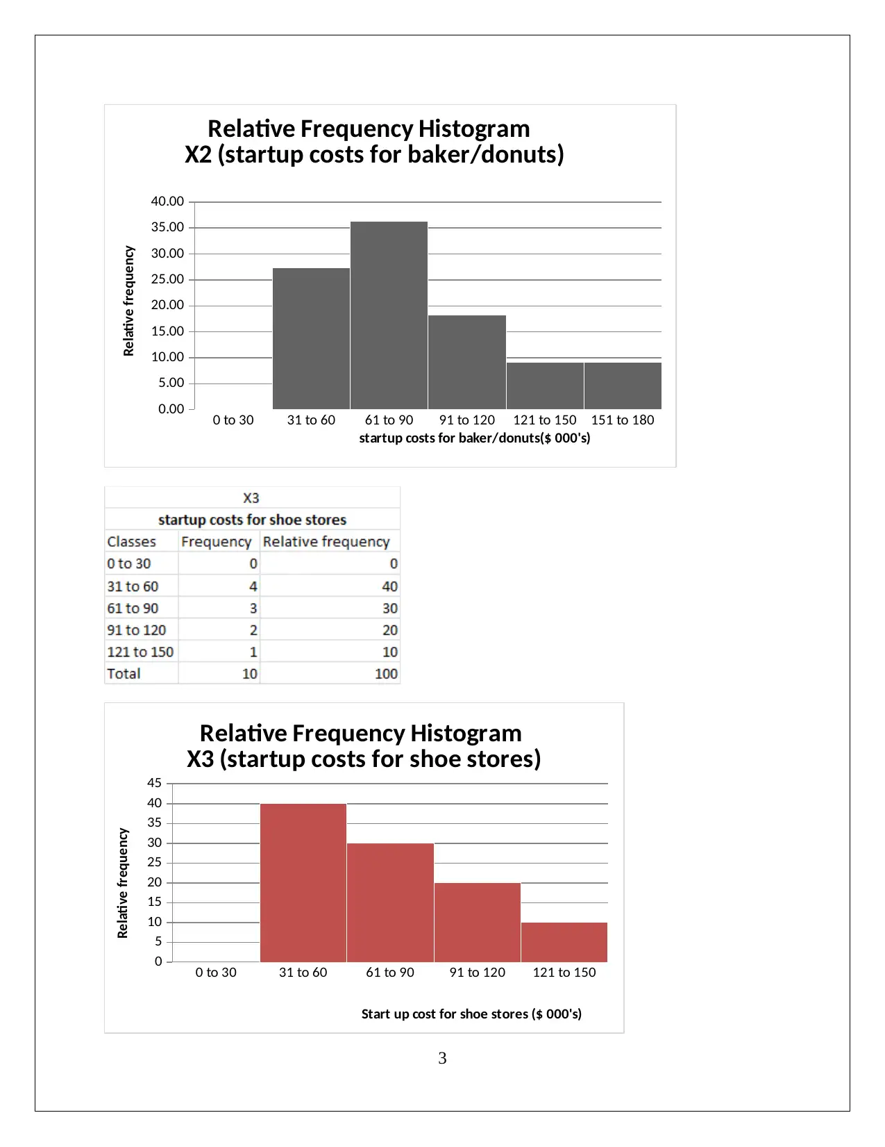
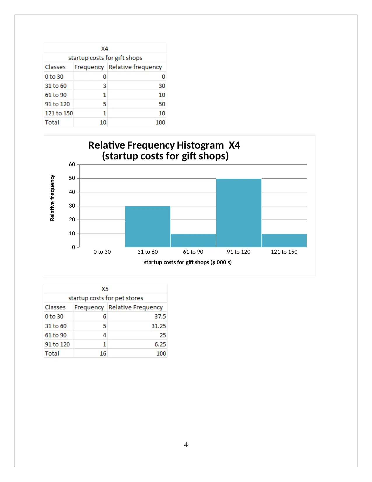
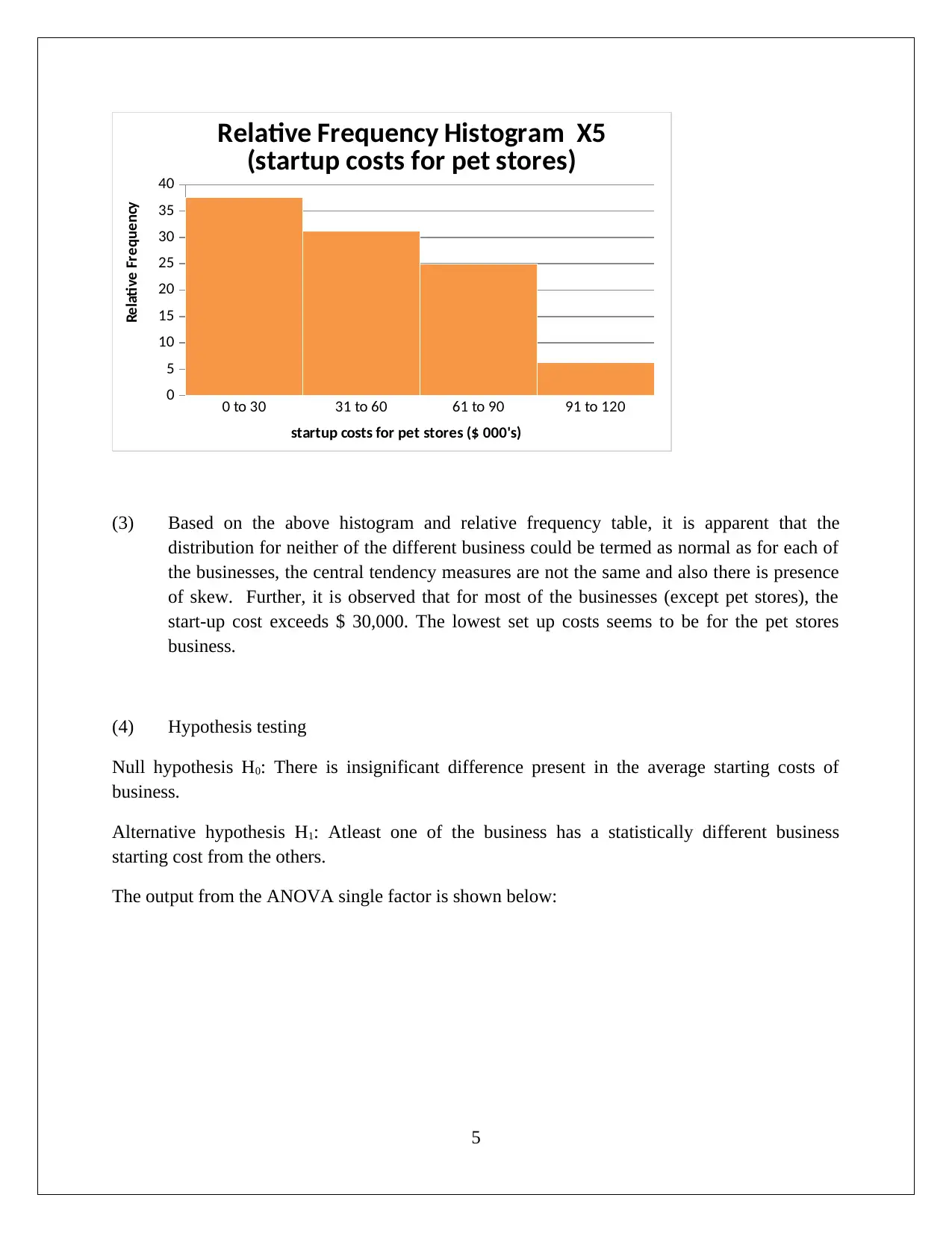
(2) The frequency and relative frequency distribution and the relative frequency histogram
for each of business type is highlighted below:
1
(1) The value of mean, median, mode , range and standard deviation for the given four type
of business is shown below:
(2) The frequency and relative frequency distribution and the relative frequency histogram
for each of business type is highlighted below:
1
0 to 30 31 to 60 61 to 90 91 to 120 121 to 150
0.00
5.00
10.00
15.00
20.00
25.00
30.00
35.00
Relative Frequency Histogram
X1 (Startup cost for Pizza)
Startup cost for pizza ($ 000's)
Relative frequency (%)
2
0.00
5.00
10.00
15.00
20.00
25.00
30.00
35.00
Relative Frequency Histogram
X1 (Startup cost for Pizza)
Startup cost for pizza ($ 000's)
Relative frequency (%)
2
⊘ This is a preview!⊘
Do you want full access?
Subscribe today to unlock all pages.

Trusted by 1+ million students worldwide
0 to 30 31 to 60 61 to 90 91 to 120 121 to 150 151 to 180
0.00
5.00
10.00
15.00
20.00
25.00
30.00
35.00
40.00
Relative Frequency Histogram
X2 (startup costs for baker/donuts)
startup costs for baker/donuts($ 000's)
Relative frequency
0 to 30 31 to 60 61 to 90 91 to 120 121 to 150
0
5
10
15
20
25
30
35
40
45
Relative Frequency Histogram
X3 (startup costs for shoe stores)
Start up cost for shoe stores ($ 000's)
Relative frequency
3
Paraphrase This Document
Need a fresh take? Get an instant paraphrase of this document with our AI Paraphraser
0 to 30 31 to 60 61 to 90 91 to 120 121 to 150
0
10
20
30
40
50
60
Relative Frequency Histogram X4
(startup costs for gift shops)
startup costs for gift shops ($ 000's)
Relative frequency
4
0
10
20
30
40
50
60
Relative Frequency Histogram X4
(startup costs for gift shops)
startup costs for gift shops ($ 000's)
Relative frequency
4
0 to 30 31 to 60 61 to 90 91 to 120
0
5
10
15
20
25
30
35
40
Relative Frequency Histogram X5
(startup costs for pet stores)
startup costs for pet stores ($ 000's)
Relative Frequency
(3) Based on the above histogram and relative frequency table, it is apparent that the
distribution for neither of the different business could be termed as normal as for each of
the businesses, the central tendency measures are not the same and also there is presence
of skew. Further, it is observed that for most of the businesses (except pet stores), the
start-up cost exceeds $ 30,000. The lowest set up costs seems to be for the pet stores
business.
(4) Hypothesis testing
Null hypothesis H0: There is insignificant difference present in the average starting costs of
business.
Alternative hypothesis H1: Atleast one of the business has a statistically different business
starting cost from the others.
The output from the ANOVA single factor is shown below:
5
⊘ This is a preview!⊘
Do you want full access?
Subscribe today to unlock all pages.

Trusted by 1+ million students worldwide
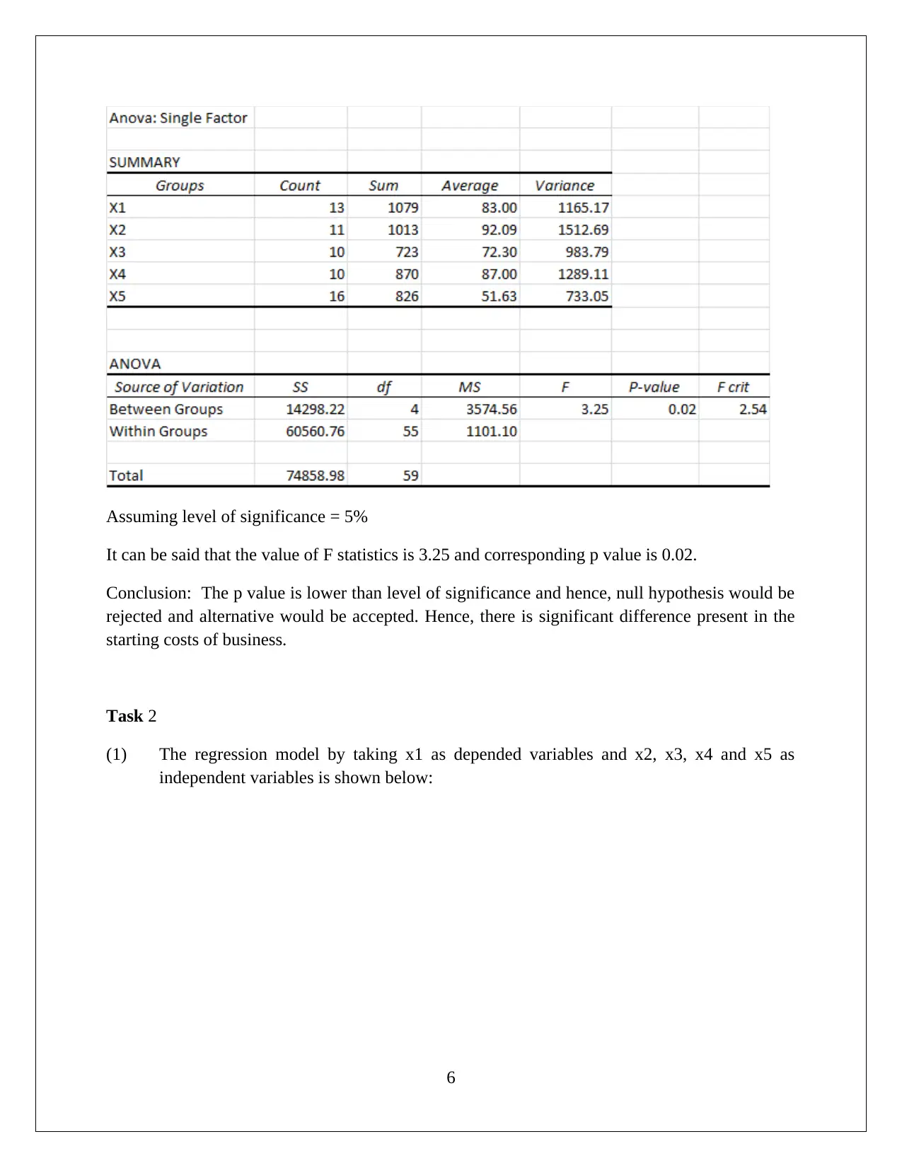
Assuming level of significance = 5%
It can be said that the value of F statistics is 3.25 and corresponding p value is 0.02.
Conclusion: The p value is lower than level of significance and hence, null hypothesis would be
rejected and alternative would be accepted. Hence, there is significant difference present in the
starting costs of business.
Task 2
(1) The regression model by taking x1 as depended variables and x2, x3, x4 and x5 as
independent variables is shown below:
6
Paraphrase This Document
Need a fresh take? Get an instant paraphrase of this document with our AI Paraphraser
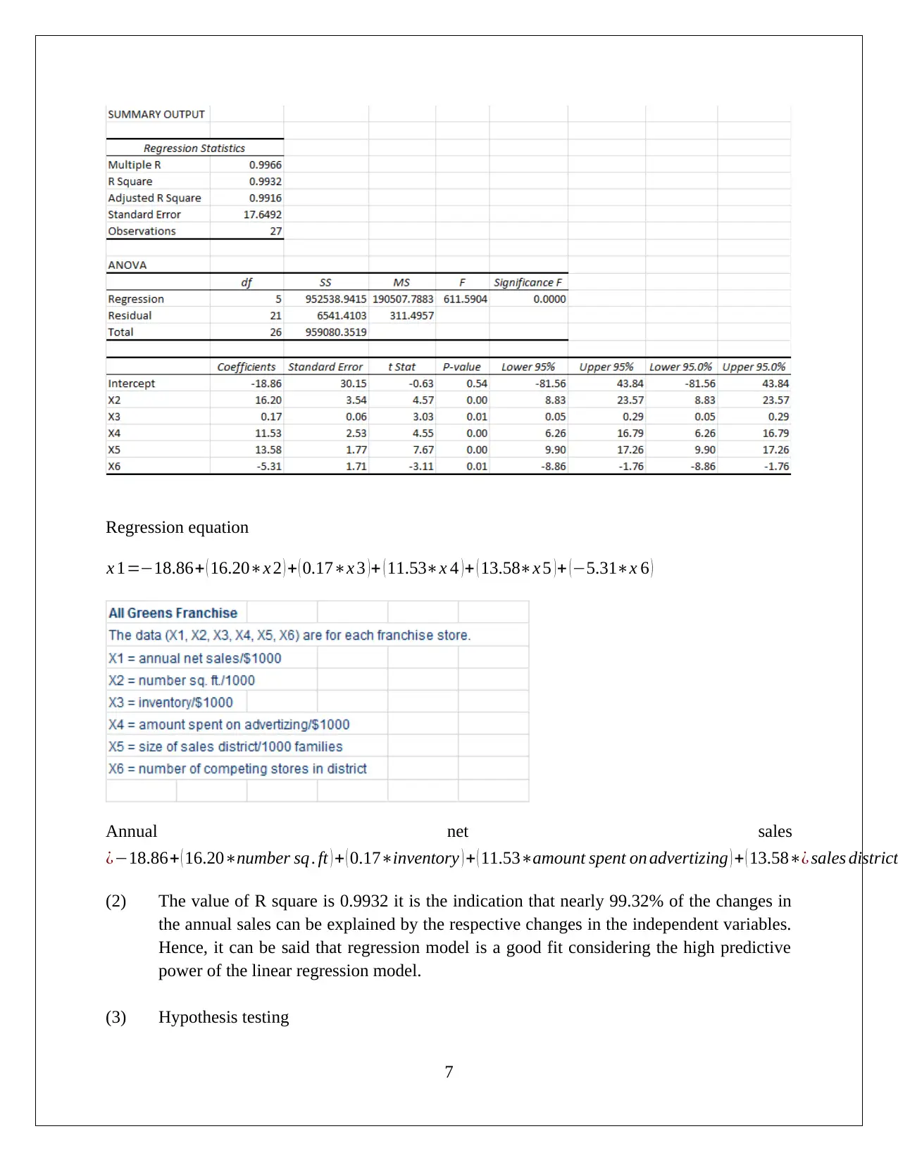
Regression equation
x 1=−18.86+ ( 16.20∗x 2 ) + ( 0.17∗x 3 )+ ( 11.53∗x 4 )+ ( 13.58∗x 5 )+ (−5.31∗x 6 )
Annual net sales
¿−18.86+ ( 16.20∗number sq . ft ) + ( 0.17∗inventory ) + ( 11.53∗amount spent on advertizing ) + ( 13.58∗¿ sales district
(2) The value of R square is 0.9932 it is the indication that nearly 99.32% of the changes in
the annual sales can be explained by the respective changes in the independent variables.
Hence, it can be said that regression model is a good fit considering the high predictive
power of the linear regression model.
(3) Hypothesis testing
7
Null hypothesis H0: All the slopes can be assumed to be zero.
Alternative hypothesis H1: Atleast one of the slopes is not equal to zero.
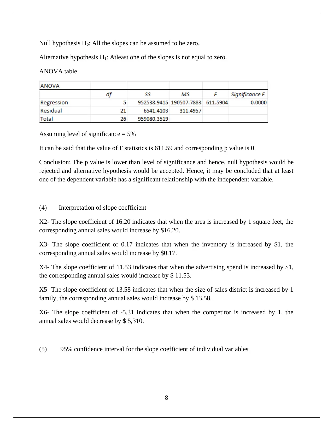
ANOVA table
Assuming level of significance = 5%
It can be said that the value of F statistics is 611.59 and corresponding p value is 0.
Conclusion: The p value is lower than level of significance and hence, null hypothesis would be
rejected and alternative hypothesis would be accepted. Hence, it may be concluded that at least
one of the dependent variable has a significant relationship with the independent variable.
(4) Interpretation of slope coefficient
X2- The slope coefficient of 16.20 indicates that when the area is increased by 1 square feet, the
corresponding annual sales would increase by $16.20.
X3- The slope coefficient of 0.17 indicates that when the inventory is increased by $1, the
corresponding annual sales would increase by $0.17.
X4- The slope coefficient of 11.53 indicates that when the advertising spend is increased by $1,
the corresponding annual sales would increase by $ 11.53.
X5- The slope coefficient of 13.58 indicates that when the size of sales district is increased by 1
family, the corresponding annual sales would increase by $ 13.58.
X6- The slope coefficient of -5.31 indicates that when the competitor is increased by 1, the
annual sales would decrease by $ 5,310.
(5) 95% confidence interval for the slope coefficient of individual variables
8
⊘ This is a preview!⊘
Do you want full access?
Subscribe today to unlock all pages.

Trusted by 1+ million students worldwide
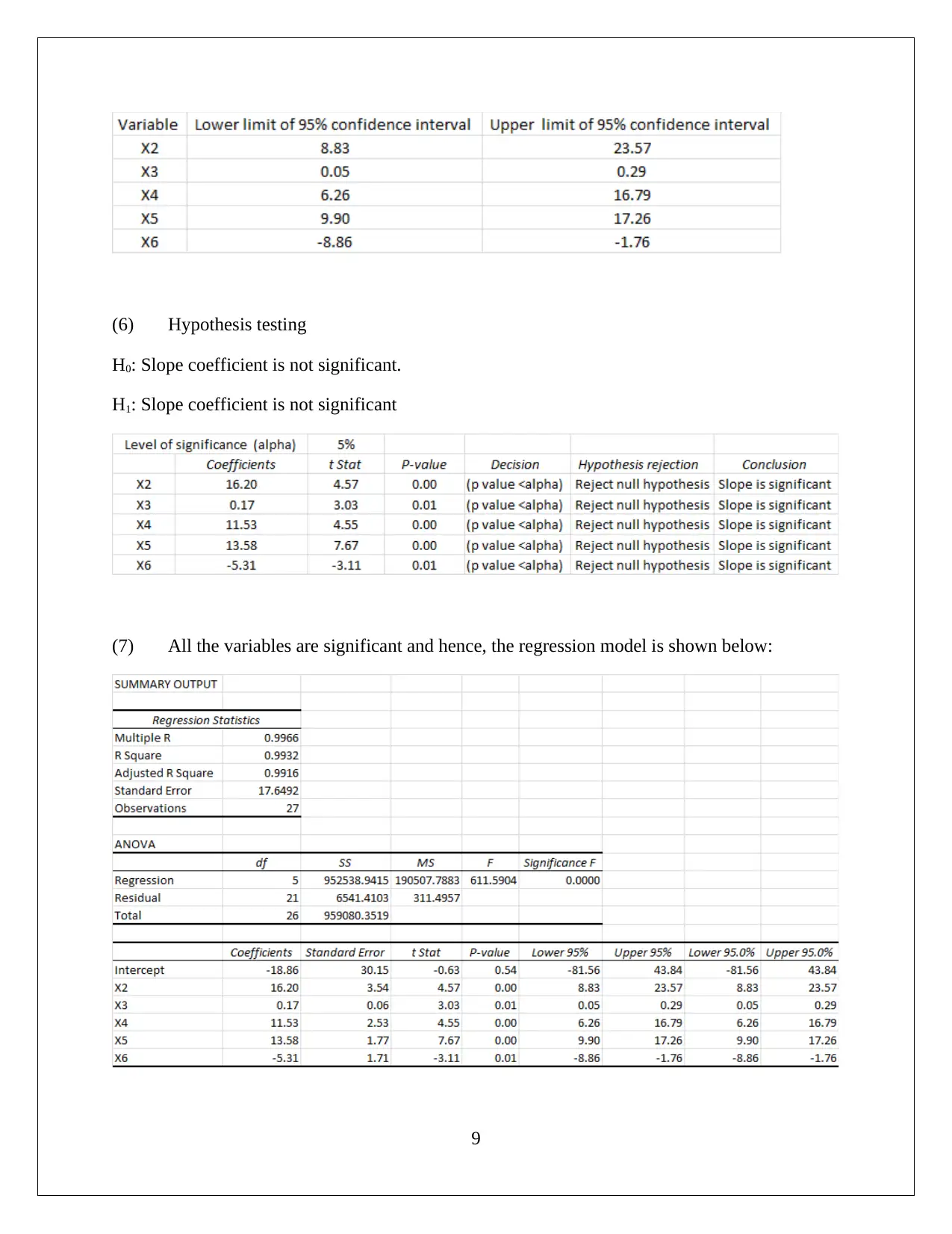
(6) Hypothesis testing
H0: Slope coefficient is not significant.
H1: Slope coefficient is not significant
(7) All the variables are significant and hence, the regression model is shown below:
9
H0: Slope coefficient is not significant.
H1: Slope coefficient is not significant
(7) All the variables are significant and hence, the regression model is shown below:
9
Paraphrase This Document
Need a fresh take? Get an instant paraphrase of this document with our AI Paraphraser
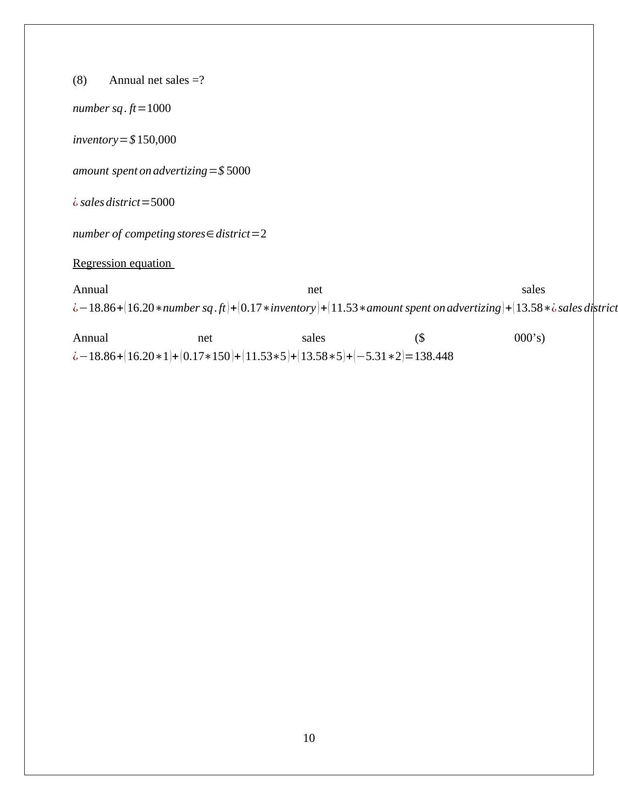
(8) Annual net sales =?
number sq . ft=1000
inventory=$ 150,000
amount spent on advertizing=$ 5000
¿ sales district=5000
number of competing stores∈ district=2
Regression equation
Annual net sales
¿−18.86+ ( 16.20∗number sq . ft ) + ( 0.17∗inventory ) + ( 11.53∗amount spent on advertizing ) + ( 13.58∗¿ sales district
Annual net sales ($ 000’s)
¿−18.86+ ( 16.20∗1 )+ ( 0.17∗150 )+ ( 11.53∗5 )+ ( 13.58∗5 ) + (−5.31∗2 )=138.448
10
1 out of 11
Related Documents
Your All-in-One AI-Powered Toolkit for Academic Success.
+13062052269
info@desklib.com
Available 24*7 on WhatsApp / Email
![[object Object]](/_next/static/media/star-bottom.7253800d.svg)
Unlock your academic potential
Copyright © 2020–2026 A2Z Services. All Rights Reserved. Developed and managed by ZUCOL.


