Analysis of Study Material on Desklib

This document provides a comprehensive analysis of study material on Desklib, including statistical measures like mean, standard deviation, quartiles, probability calculations, regression analysis, and hypothesis testing. It also discusses the suitability of different statistical tests and provides conclusions based on the analysis.

Question 1
a)
Mean = 214.28
Standard Error of the Mean = 0.699574888862
Standard Deviation = 9.89348295724
Minimum = 192
Maximum = 240
First Quartile = 207
Third Quartile = 220.5
Inter-quartile Range = 13.5
Median = 214
Mode = 212

b)
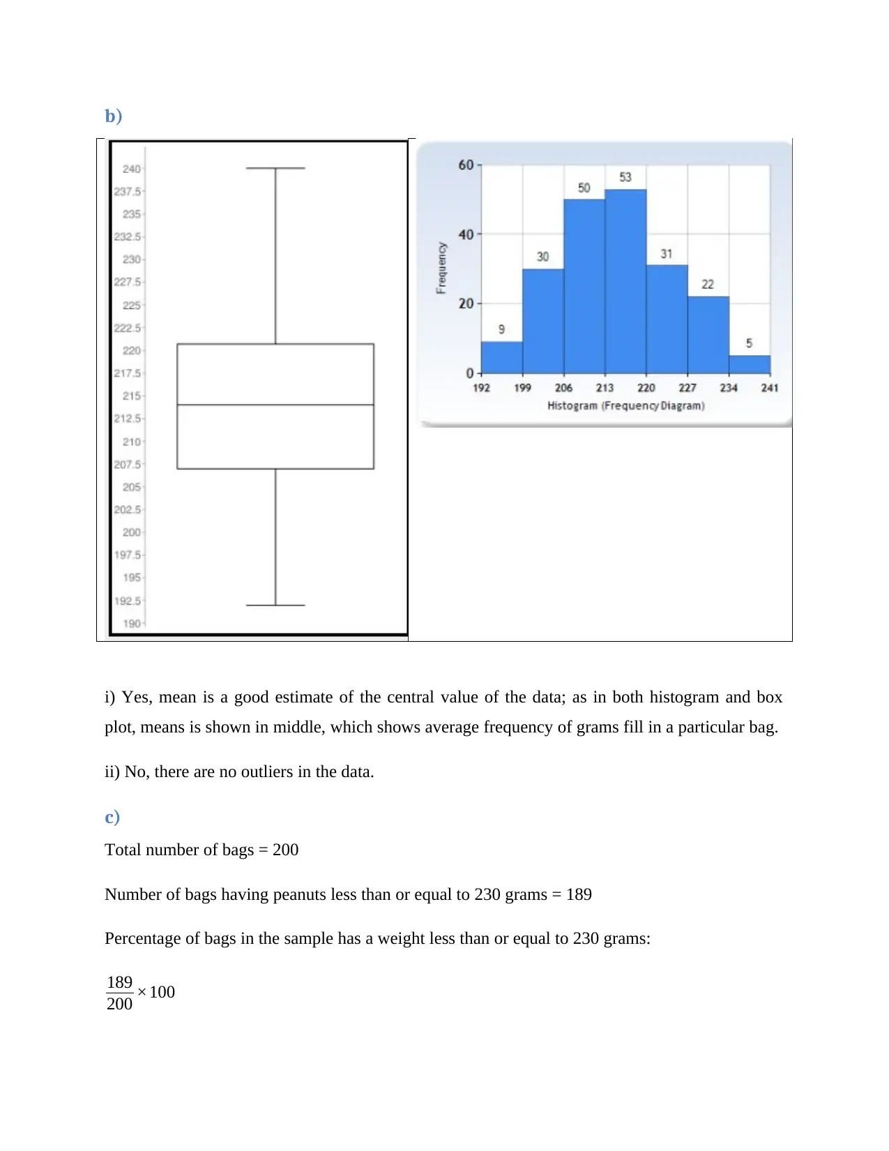
i) Yes, mean is a good estimate of the central value of the data; as in both histogram and box
plot, means is shown in middle, which shows average frequency of grams fill in a particular bag.
ii) No, there are no outliers in the data.
c)
Total number of bags = 200
Number of bags having peanuts less than or equal to 230 grams = 189
Percentage of bags in the sample has a weight less than or equal to 230 grams:
189
200 ×100

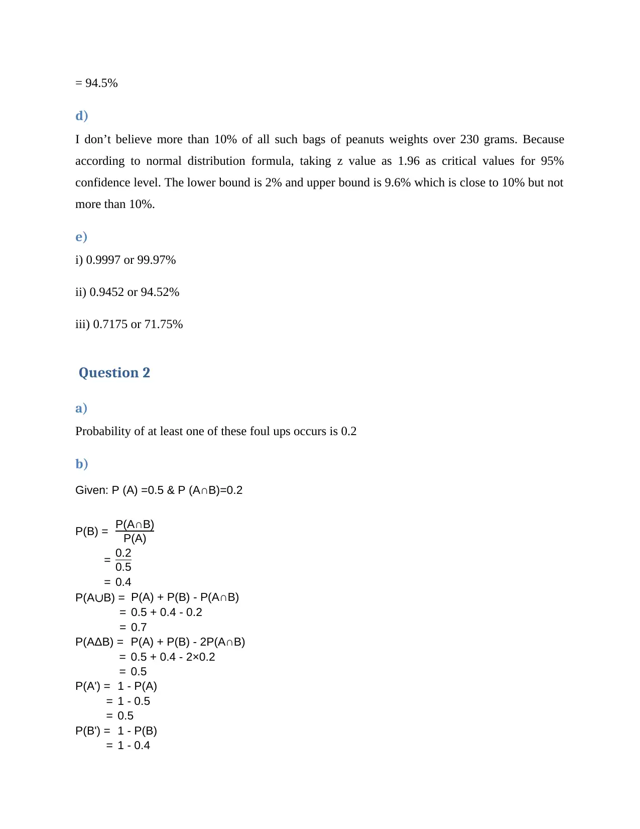
= 94.5%
d)
I don’t believe more than 10% of all such bags of peanuts weights over 230 grams. Because
according to normal distribution formula, taking z value as 1.96 as critical values for 95%
confidence level. The lower bound is 2% and upper bound is 9.6% which is close to 10% but not
more than 10%.
e)
i) 0.9997 or 99.97%
ii) 0.9452 or 94.52%
iii) 0.7175 or 71.75%
Question 2
a)
Probability of at least one of these foul ups occurs is 0.2
b)
Given: P (A) =0.5 & P (A∩B)=0.2
P(B) = P(A∩B)
P(A)
= 0.2
0.5
= 0.4
P(A∪B) = P(A) + P(B) - P(A∩B)
= 0.5 + 0.4 - 0.2
= 0.7
P(AΔB) = P(A) + P(B) - 2P(A∩B)
= 0.5 + 0.4 - 2×0.2
= 0.5
P(A') = 1 - P(A)
= 1 - 0.5
= 0.5
P(B') = 1 - P(B)
= 1 - 0.4

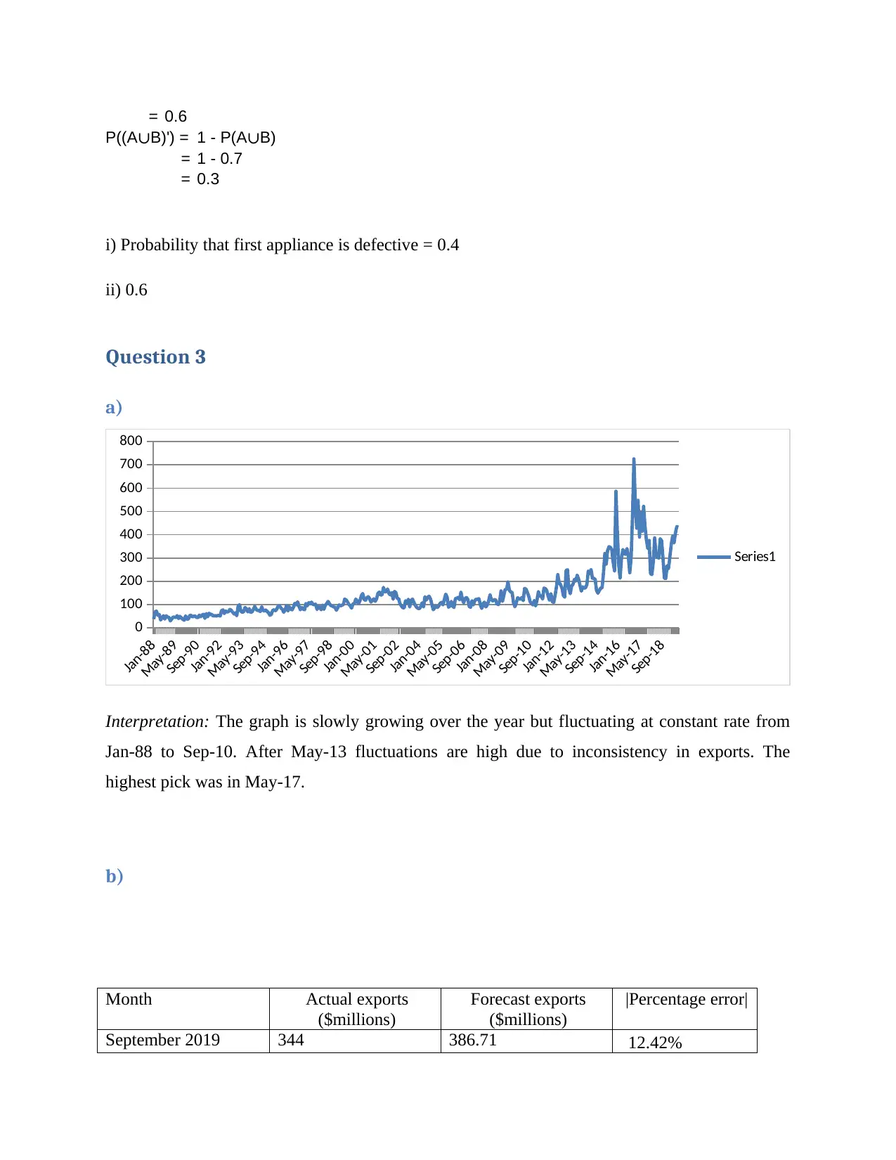
= 0.6
P((A∪B)') = 1 - P(A∪B)
= 1 - 0.7
= 0.3
i) Probability that first appliance is defective = 0.4
ii) 0.6
Question 3
a)
Jan-88
May-89
Sep-90
Jan-92
May-93
Sep-94
Jan-96
May-97
Sep-98
Jan-00
May-01
Sep-02
Jan-04
May-05
Sep-06
Jan-08
May-09
Sep-10
Jan-12
May-13
Sep-14
Jan-16
May-17
Sep-18
0
100
200
300
400
500
600
700
800
Series1
Interpretation: The graph is slowly growing over the year but fluctuating at constant rate from
Jan-88 to Sep-10. After May-13 fluctuations are high due to inconsistency in exports. The
highest pick was in May-17.
b)
Month Actual exports
($millions)
Forecast exports
($millions)
|Percentage error|
September 2019 344 386.71 12.42%

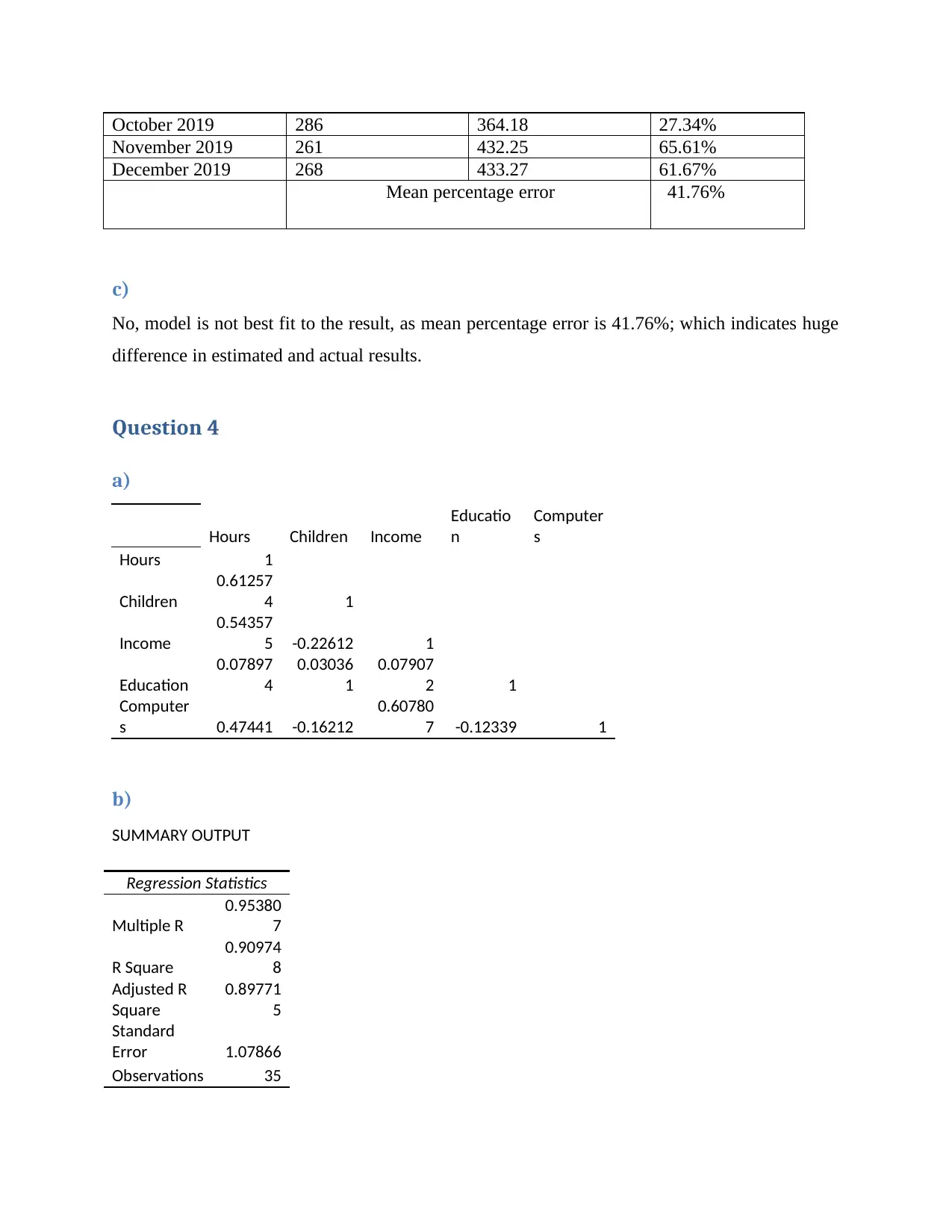
October 2019 286 364.18 27.34%
November 2019 261 432.25 65.61%
December 2019 268 433.27 61.67%
Mean percentage error 41.76%
c)
No, model is not best fit to the result, as mean percentage error is 41.76%; which indicates huge
difference in estimated and actual results.
Question 4
a)
Hours Children Income
Educatio
n
Computer
s
Hours 1
Children
0.61257
4 1
Income
0.54357
5 -0.22612 1
Education
0.07897
4
0.03036
1
0.07907
2 1
Computer
s 0.47441 -0.16212
0.60780
7 -0.12339 1
b)
SUMMARY OUTPUT
Regression Statistics
Multiple R
0.95380
7
R Square
0.90974
8
Adjusted R
Square
0.89771
5
Standard
Error 1.07866
Observations 35

ANOVA
df SS MS F
Significan
ce F
Regression 4 351.8484
87.96
21
75.60
082 3.14E-15
Residual 30 34.90521
1.163
507
Total 34 386.7536
Coefficie
nts
Standard
Error t Stat
P-
value
Lower
95%
Upper
95%
Lower
95.0%
Upper
95.0%
Intercept
3.50042
8 1.972015
1.775
051
0.086
037 -0.52696
7.5278
2 -0.52696 7.52782
Children 2.15671 0.155944
13.83
007
1.49E-
14 1.838231
2.4751
89
1.83823
1 2.475189
Income
0.00012
6 1.64E-05
7.719
069
1.3E-
08 9.3E-05
0.0001
6 9.3E-05 0.00016
Education
0.12199
8 0.152432
0.800
347
0.429
803 -0.18931
0.4333
06 -0.18931 0.433306
Computers
2.26537
8 0.591134
3.832
256
0.000
604 1.058121
3.4726
35
1.05812
1 3.472635
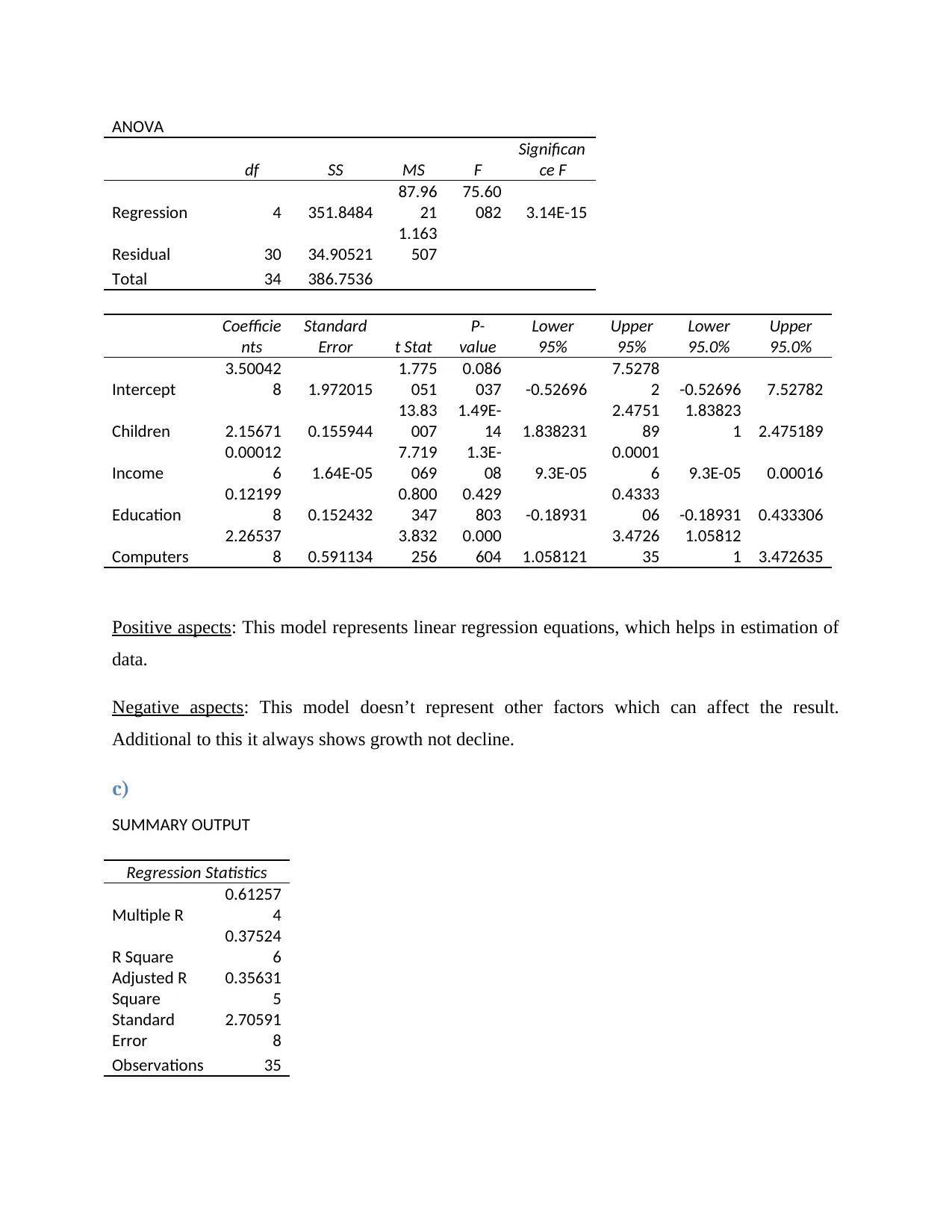
Positive aspects: This model represents linear regression equations, which helps in estimation of
data.
Negative aspects: This model doesn’t represent other factors which can affect the result.
Additional to this it always shows growth not decline.
c)
SUMMARY OUTPUT
Regression Statistics
Multiple R
0.61257
4
R Square
0.37524
6
Adjusted R
Square
0.35631
5
Standard
Error
2.70591
8
Observations 35

ANOVA
df SS MS F
Significan
ce F
Regression 1 145.1279
145.1
279
19.82
083 9.18E-05
Residual 33 241.6257
7.321
99
Total 34 386.7536
Coefficie
nts
Standard
Error t Stat
P-
value
Lower
95%
Upper
95%
Lower
95.0%
Upper
95.0%
Intercept
11.9898
5 0.710408
16.87
741
8.52E-
18 10.54451
13.435
18
10.5445
1 13.43518
Children
1.69403
7 0.380506
4.452
059
9.18E-
05 0.919891
2.4681
83
0.91989
1 2.468183
PROBABILITY OUTPUT
Percentile Hours
1.428571
9.39881
6
4.285714 9.86857
7.142857
10.2233
5
10
10.4402
9
12.85714
10.5823
9
15.71429
10.6397
1
18.57143
10.8438
2
21.42857
11.0076
3
24.28571
11.3606
5
27.14286 11.6457
30
11.7418
9
32.85714
12.4384
6
35.71429
12.8836
6
38.57143 13.0019

41.42857
13.1030
3
44.28571
13.6791
1
47.14286
13.9994
8
50
14.0295
4
52.85714
15.1846
9
55.71429
15.2044
3
58.57143
15.2580
6
61.42857 15.3199
64.28571
15.3295
4
67.14286
15.5574
9
70
16.3032
1
72.85714
16.6623
8
75.71429 16.6639
78.57143
17.0199
5
81.42857
17.2100
9
84.28571
17.7445
5
87.14286
18.3053
6
90
18.8198
3
92.85714
19.3989
8
95.71429
19.6890
7
98.57143
23.7870
2
d)
Hours Children Income
Educatio
n
Computer
s
Hours 11.0501

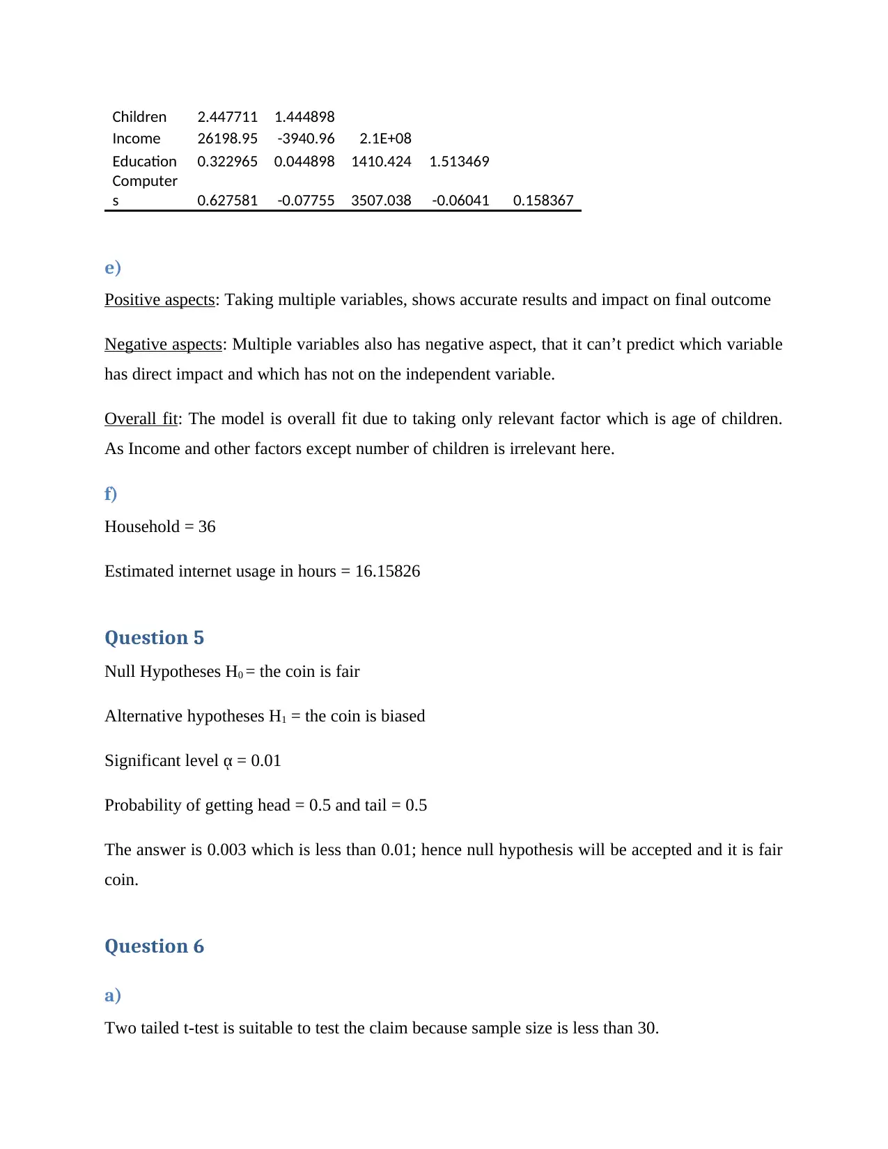
Children 2.447711 1.444898
Income 26198.95 -3940.96 2.1E+08
Education 0.322965 0.044898 1410.424 1.513469
Computer
s 0.627581 -0.07755 3507.038 -0.06041 0.158367
e)
Positive aspects: Taking multiple variables, shows accurate results and impact on final outcome
Negative aspects: Multiple variables also has negative aspect, that it can’t predict which variable
has direct impact and which has not on the independent variable.
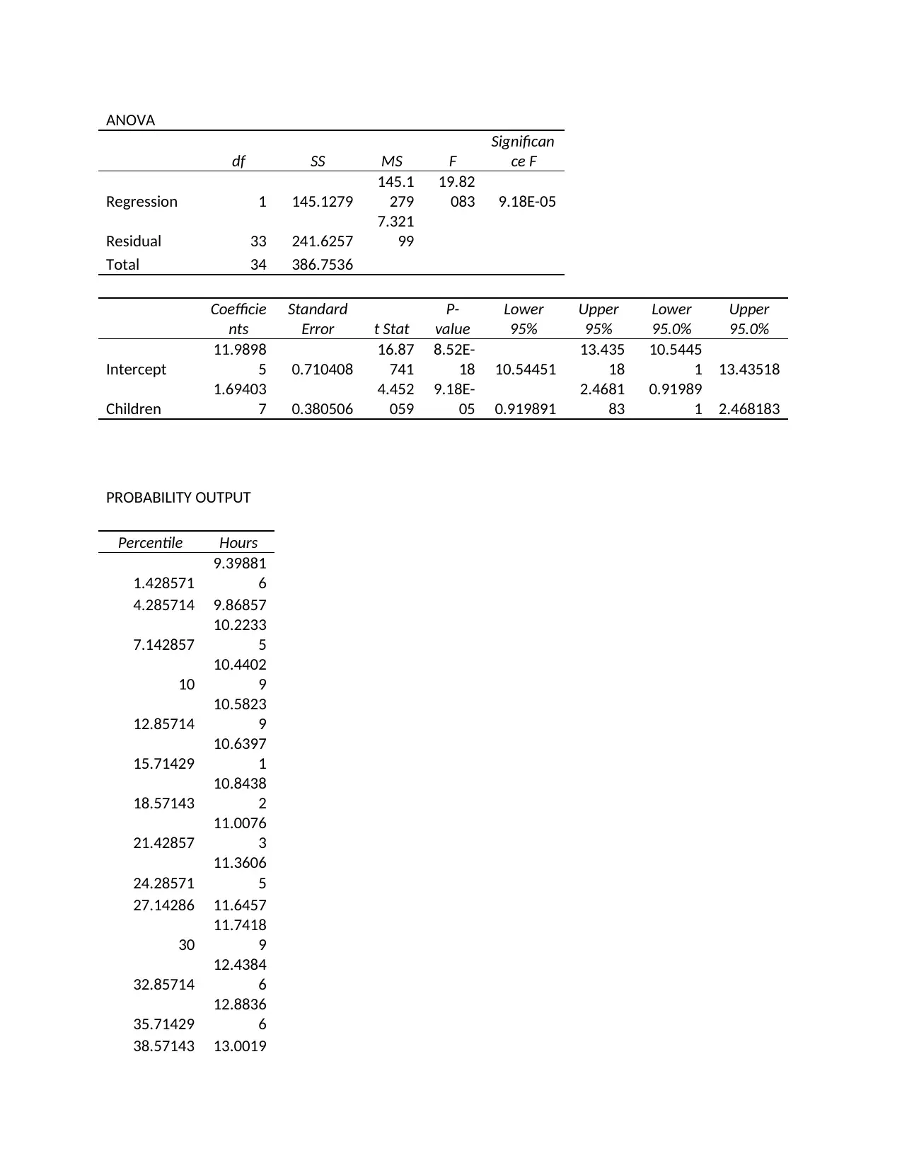
Overall fit: The model is overall fit due to taking only relevant factor which is age of children.
As Income and other factors except number of children is irrelevant here.
f)
Household = 36
Estimated internet usage in hours = 16.15826
Question 5
Null Hypotheses H0 = the coin is fair
Alternative hypotheses H1 = the coin is biased
Significant level ᾳ = 0.01
Probability of getting head = 0.5 and tail = 0.5
The answer is 0.003 which is less than 0.01; hence null hypothesis will be accepted and it is fair
coin.
Question 6
a)
Two tailed t-test is suitable to test the claim because sample size is less than 30.

b)
Null Hypotheses: Manufacturer place an average of 75 chocolate chips in a tub
Alternative hypotheses: Manufacturer is not placing an average of 75 chocolate chips in a one
liter tub.
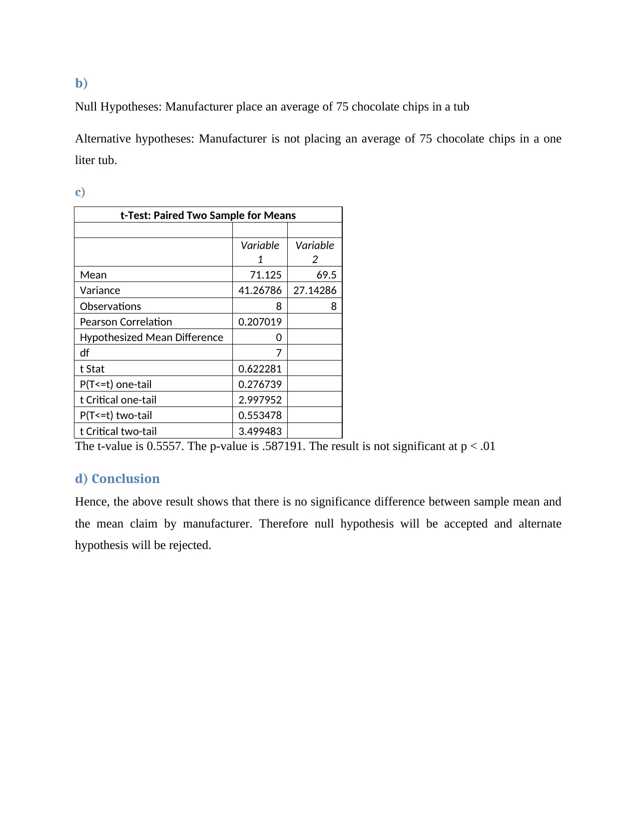
c)
t-Test: Paired Two Sample for Means
Variable
1
Variable
2
Mean 71.125 69.5
Variance 41.26786 27.14286
Observations 8 8
Pearson Correlation 0.207019
Hypothesized Mean Difference 0
df 7
t Stat 0.622281
P(T<=t) one-tail 0.276739
t Critical one-tail 2.997952
P(T<=t) two-tail 0.553478
t Critical two-tail 3.499483
The t-value is 0.5557. The p-value is .587191. The result is not significant at p < .01
d) Conclusion
Hence, the above result shows that there is no significance difference between sample mean and
the mean claim by manufacturer. Therefore null hypothesis will be accepted and alternate
hypothesis will be rejected.