Statistics Study Material

Find comprehensive study material for Statistics including solved assignments, essays, dissertations, and more on Desklib. Get expert help for your Statistics course.

STATISTICS

Question 1:
a. Provide a 95% confidence interval for all the patients who are referred to
the health centre by the hospital.
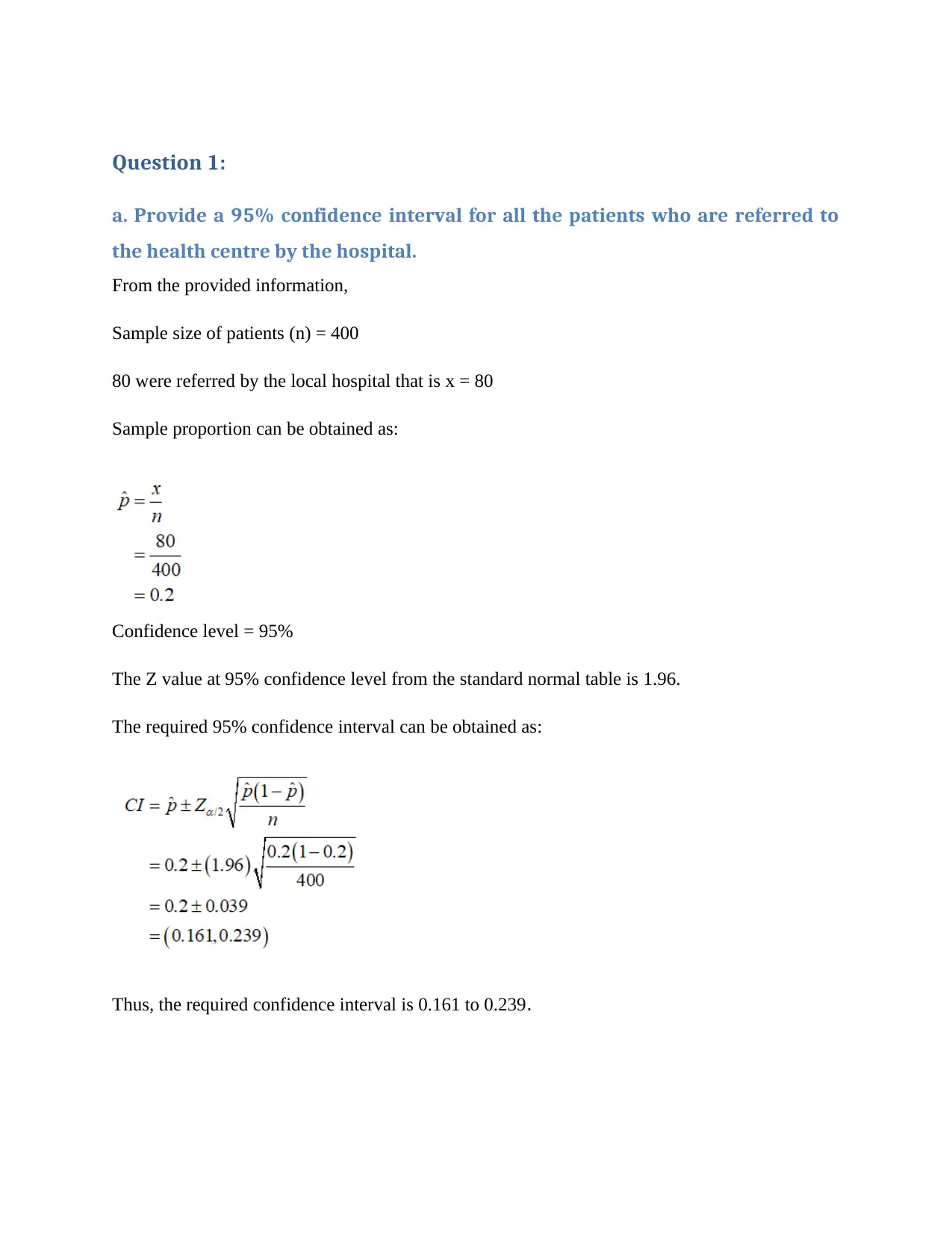
From the provided information,
Sample size of patients (n) = 400
80 were referred by the local hospital that is x = 80
Sample proportion can be obtained as:
Confidence level = 95%
The Z value at 95% confidence level from the standard normal table is 1.96.
The required 95% confidence interval can be obtained as:
Thus, the required confidence interval is 0.161 to 0.239.

b. What sample size would be required to estimate the proportion of all
hospital referrals to the health centre with a margin of error of 0.04 or less at
95% confidence?
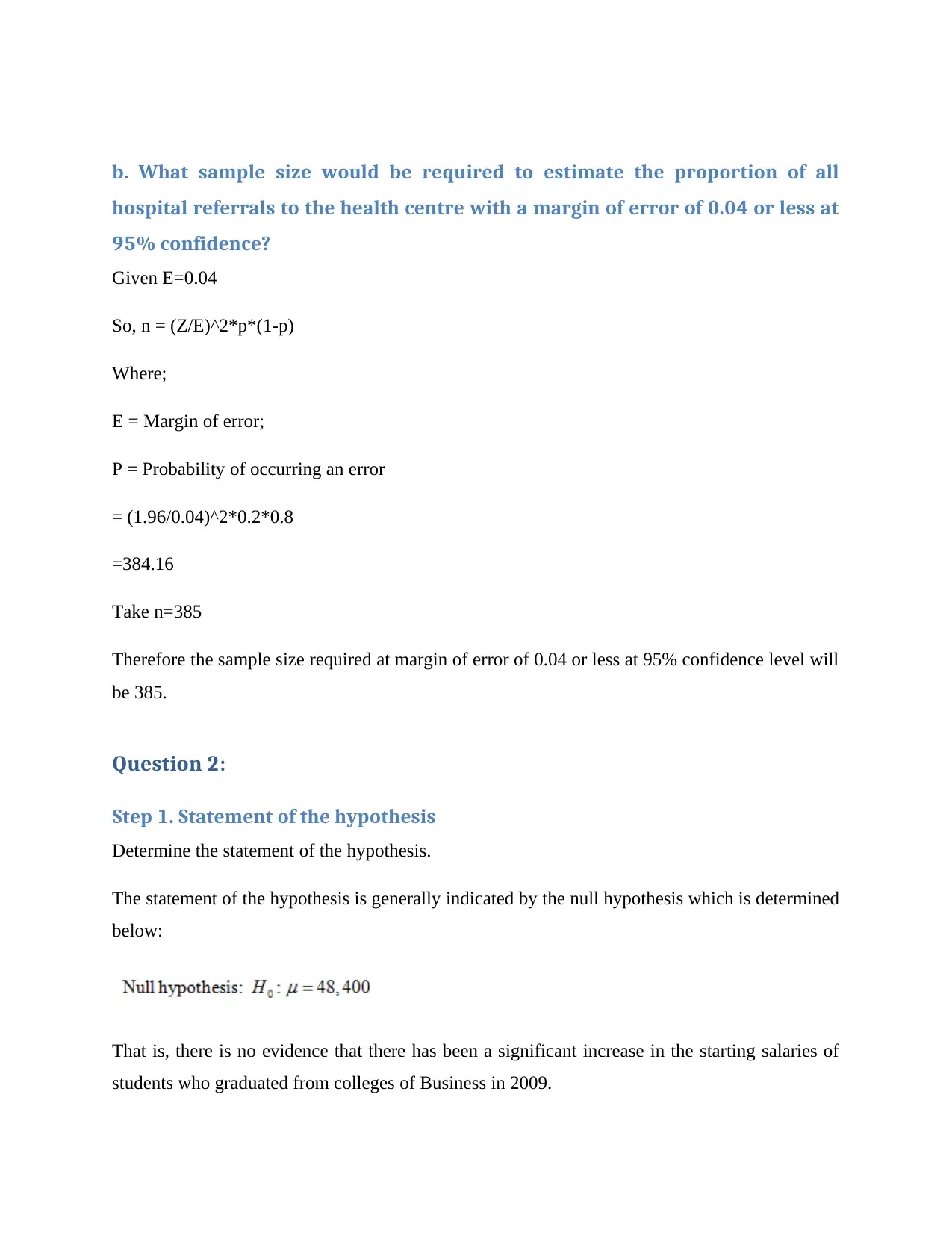
Given E=0.04
So, n = (Z/E)^2*p*(1-p)
Where;
E = Margin of error;
P = Probability of occurring an error
= (1.96/0.04)^2*0.2*0.8
=384.16
Take n=385
Therefore the sample size required at margin of error of 0.04 or less at 95% confidence level will
be 385.
Question 2:
Step 1. Statement of the hypothesis
Determine the statement of the hypothesis.
The statement of the hypothesis is generally indicated by the null hypothesis which is determined
below:
That is, there is no evidence that there has been a significant increase in the starting salaries of
students who graduated from colleges of Business in 2009.

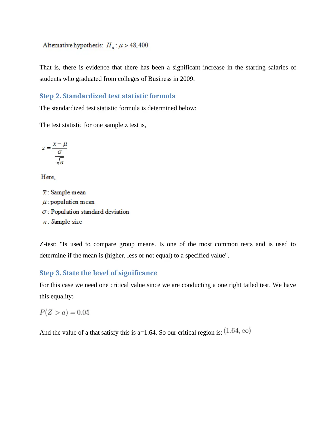
That is, there is evidence that there has been a significant increase in the starting salaries of
students who graduated from colleges of Business in 2009.
Step 2. Standardized test statistic formula
The standardized test statistic formula is determined below:
The test statistic for one sample z test is,
Z-test: "Is used to compare group means. Is one of the most common tests and is used to
determine if the mean is (higher, less or not equal) to a specified value".
Step 3. State the level of significance
For this case we need one critical value since we are conducting a one right tailed test. We have
this equality:
And the value of a that satisfy this is a=1.64. So our critical region is:

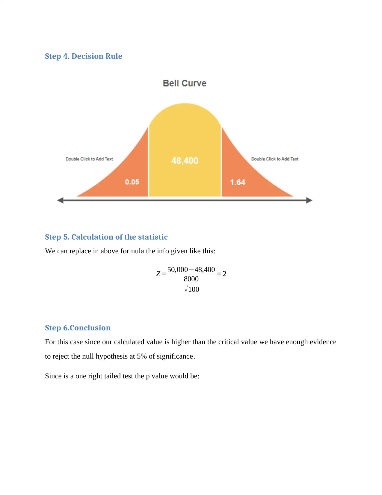
Step 4. Decision Rule
Step 5. Calculation of the statistic
We can replace in above formula the info given like this:
Z=50,000−48,400
8000
√ 100
=2
Step 6.Conclusion
For this case since our calculated value is higher than the critical value we have enough evidence
to reject the null hypothesis at 5% of significance.
Since is a one right tailed test the p value would be:

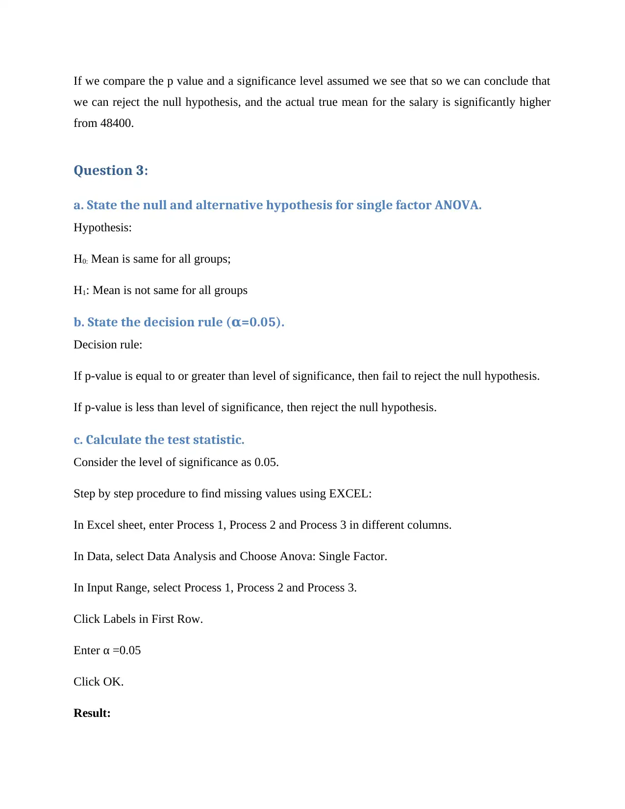
If we compare the p value and a significance level assumed we see that so we can conclude that
we can reject the null hypothesis, and the actual true mean for the salary is significantly higher
from 48400.
Question 3:
a. State the null and alternative hypothesis for single factor ANOVA.
Hypothesis:
H0: Mean is same for all groups;
H1: Mean is not same for all groups
b. State the decision rule ( =0.05).α
Decision rule:
If p-value is equal to or greater than level of significance, then fail to reject the null hypothesis.
If p-value is less than level of significance, then reject the null hypothesis.
c. Calculate the test statistic.
Consider the level of significance as 0.05.
Step by step procedure to find missing values using EXCEL:
In Excel sheet, enter Process 1, Process 2 and Process 3 in different columns.
In Data, select Data Analysis and Choose Anova: Single Factor.
In Input Range, select Process 1, Process 2 and Process 3.
Click Labels in First Row.
Enter α =0.05
Click OK.
Result:

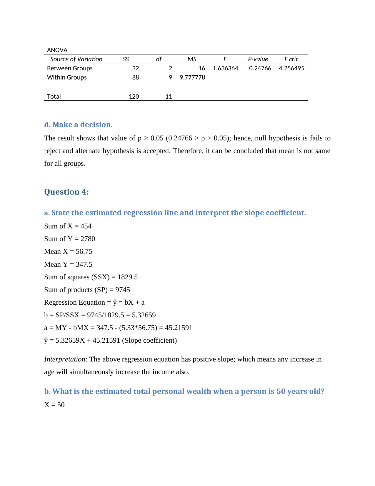
ANOVA
Source of Variation SS df MS F P-value F crit
Between Groups 32 2 16 1.636364 0.24766 4.256495
Within Groups 88 9 9.777778
Total 120 11
d. Make a decision.
The result shows that value of p ≥ 0.05 (0.24766 > p > 0.05); hence, null hypothesis is fails to
reject and alternate hypothesis is accepted. Therefore, it can be concluded that mean is not same
for all groups.
Question 4:
a. State the estimated regression line and interpret the slope coefficient.
Sum of X = 454
Sum of Y = 2780
Mean X = 56.75
Mean Y = 347.5
Sum of squares (SSX) = 1829.5
Sum of products (SP) = 9745
Regression Equation = ŷ = bX + a
b = SP/SSX = 9745/1829.5 = 5.32659
a = MY - bMX = 347.5 - (5.33*56.75) = 45.21591
ŷ = 5.32659X + 45.21591 (Slope coefficient)
Interpretation: The above regression equation has positive slope; which means any increase in
age will simultaneously increase the income also.
b. What is the estimated total personal wealth when a person is 50 years old?
X = 50

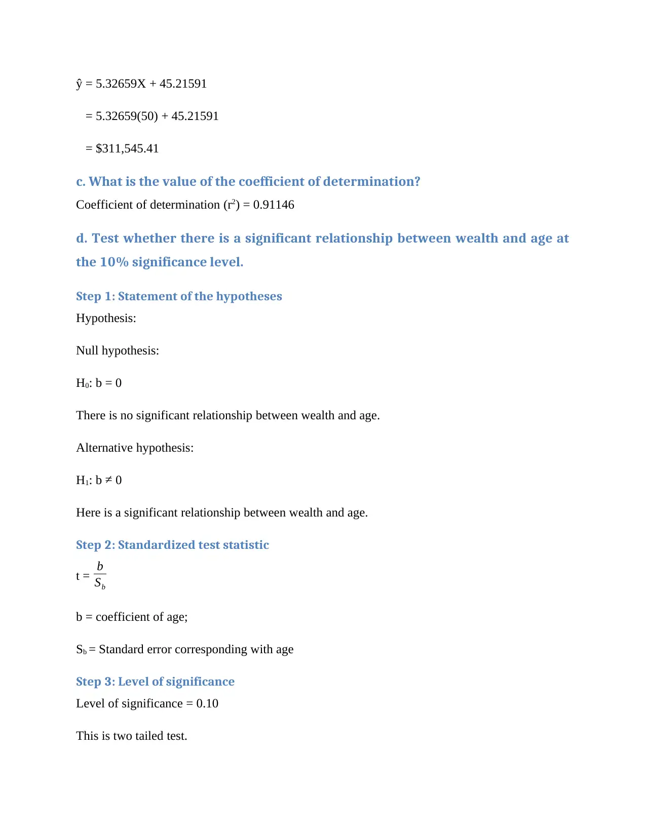
ŷ = 5.32659X + 45.21591
= 5.32659(50) + 45.21591
= $311,545.41
c. What is the value of the coefficient of determination?
Coefficient of determination (r2) = 0.91146
d. Test whether there is a significant relationship between wealth and age at
the 10% significance level.
Step 1: Statement of the hypotheses
Hypothesis:
Null hypothesis:
H0: b = 0
There is no significant relationship between wealth and age.
Alternative hypothesis:
H1: b ≠ 0
Here is a significant relationship between wealth and age.
Step 2: Standardized test statistic
t = b
Sb
b = coefficient of age;
Sb = Standard error corresponding with age
Step 3: Level of significance
Level of significance = 0.10
This is two tailed test.

Step 4: Decision Rule
If the value of p is equal to or more than 0.10; than H0 will be rejected and H1 will be accepted.
Step 5: Calculation of test statistic
t = 5.3265/0.6777
t = 7.859
p = 0.003967
Step 6: Conclusion
The value of p < 0.10 (0.003967 < p < 0.10); hence H0 is accepted and therefore it can be
concluded that there is no significant relationship between wealth and age.
Question 5:
a. Write out the estimated regression equation for the relationship between
the variables.
Multiple linear regression models:
A multiple linear regression model is given as y^ = b0 + b1x1 +…+ bkxk where y^ is the
predicted value of response variable, and x1, x2,…,xk are the k predictor variables. The
quantities b1, b2,…,bk are the estimated slopes corresponding to x1, x2,…,xk respectively. b0 is
the estimated intercept of the line, from the sample data.
Here, the dependent variable is Family spending (Y) and the independent variables are income
(X1), Family size (X2) and additions to savings (X3).
From the given regression output, the multiple linear regression model is as given below:
Y = 0.0136 + 0.7992X1 + 0.228X2 – 0.5796X3.

b. Compute coefficient of determination. What can you say about the strength
of this relationship?
Coefficient of Determination:
It is denoted by r2, here r represents the correlation between the two variables.
The r2 value represents the proportion of variation in the dependent variable explained by the
independent variable.
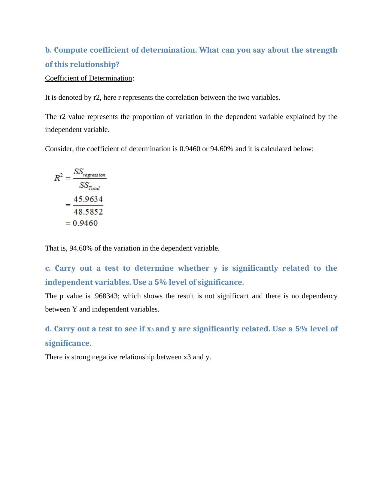
Consider, the coefficient of determination is 0.9460 or 94.60% and it is calculated below:
That is, 94.60% of the variation in the dependent variable.
c. Carry out a test to determine whether y is significantly related to the
independent variables. Use a 5% level of significance.
The p value is .968343; which shows the result is not significant and there is no dependency
between Y and independent variables.
d. Carry out a test to see if x3 and y are significantly related. Use a 5% level of
significance.
There is strong negative relationship between x3 and y.