Bankruptcy Analysis & Statistical Hypothesis
VerifiedAdded on 2020/04/01
|20
|1332
|42
AI Summary
This assignment delves into the analysis of financial data related to bankrupt and non-bankrupt firms. It requires students to assess the normality of the variables using plots, determine 95% confidence intervals, and conduct hypothesis testing to identify statistically significant differences between the two groups for various financial metrics. The analysis utilizes statistical methods and software tools like Excel's KADD add-in.
Contribute Materials
Your contribution can guide someone’s learning journey. Share your
documents today.
Statistics For Management Decision
Assessment -II
Student id and name
[Pick the date]
Assessment -II
Student id and name
[Pick the date]
Secure Best Marks with AI Grader
Need help grading? Try our AI Grader for instant feedback on your assignments.
Question 1
Selected name of the companies which are listed in Australian Stock Exchange
CWN.ASX
TAH.ASX
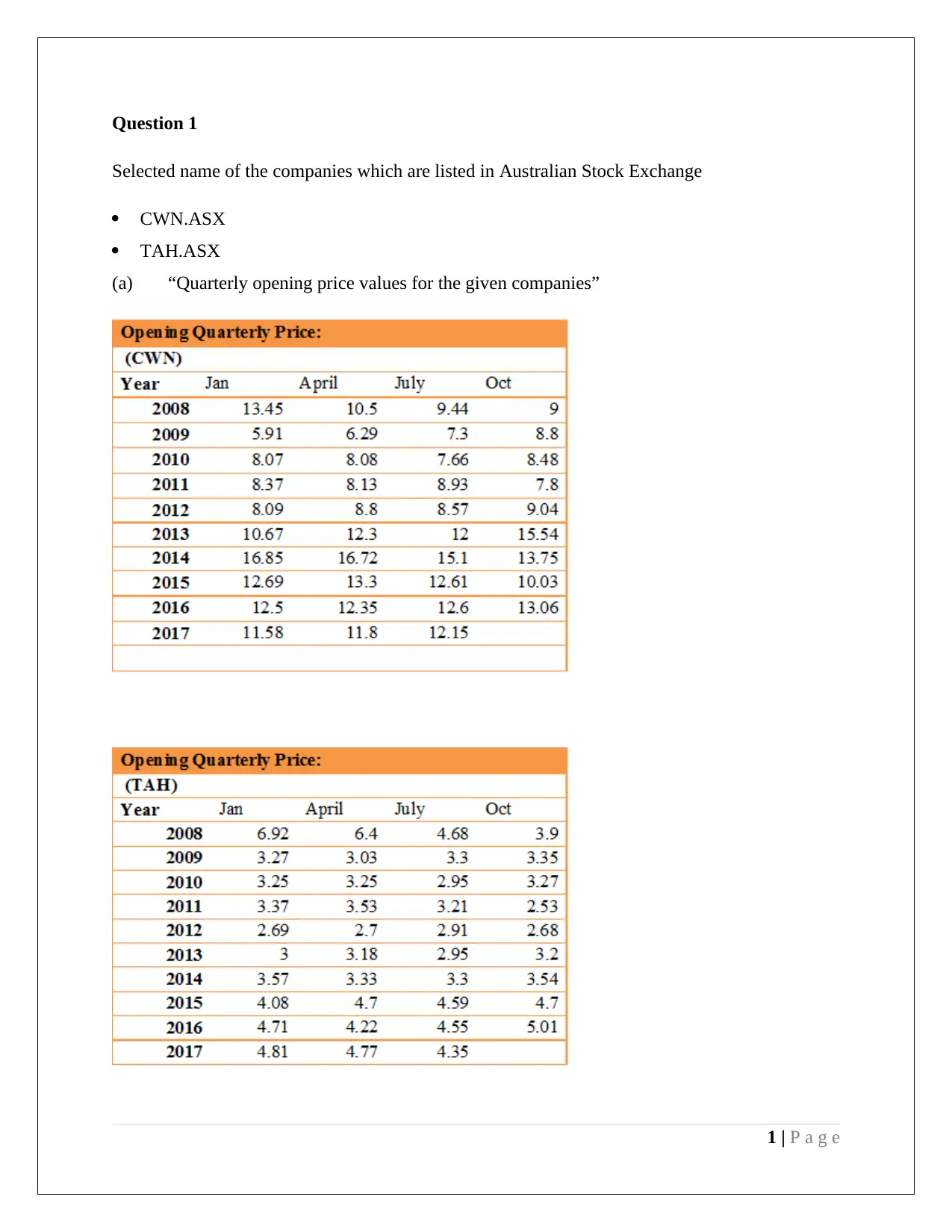
(a) “Quarterly opening price values for the given companies”
1 | P a g e
Selected name of the companies which are listed in Australian Stock Exchange
CWN.ASX
TAH.ASX
(a) “Quarterly opening price values for the given companies”
1 | P a g e
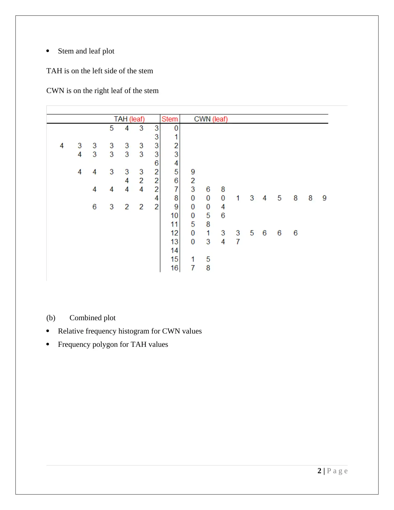
Stem and leaf plot
TAH is on the left side of the stem
CWN is on the right leaf of the stem
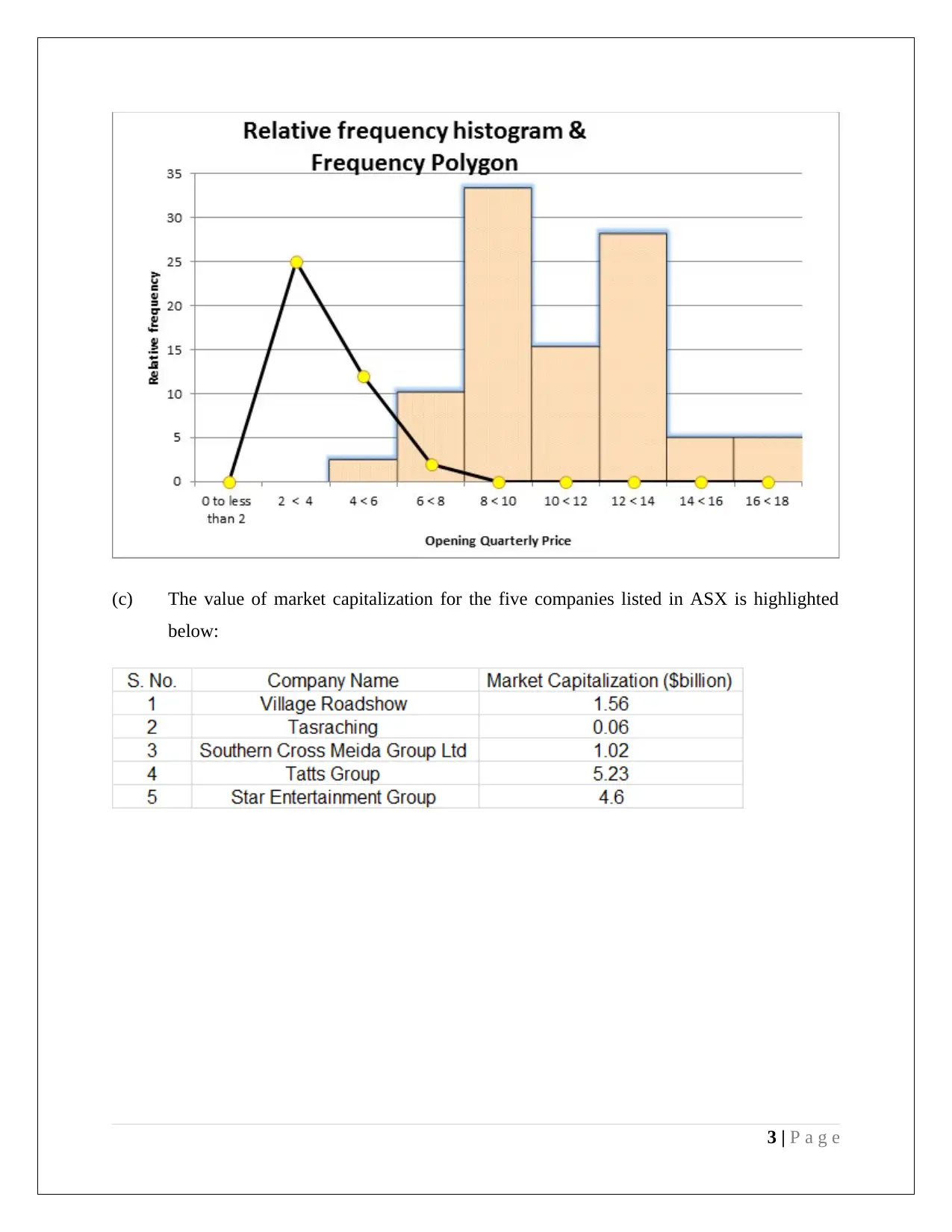
(b) Combined plot
Relative frequency histogram for CWN values
Frequency polygon for TAH values
2 | P a g e
TAH is on the left side of the stem
CWN is on the right leaf of the stem
(b) Combined plot
Relative frequency histogram for CWN values
Frequency polygon for TAH values
2 | P a g e
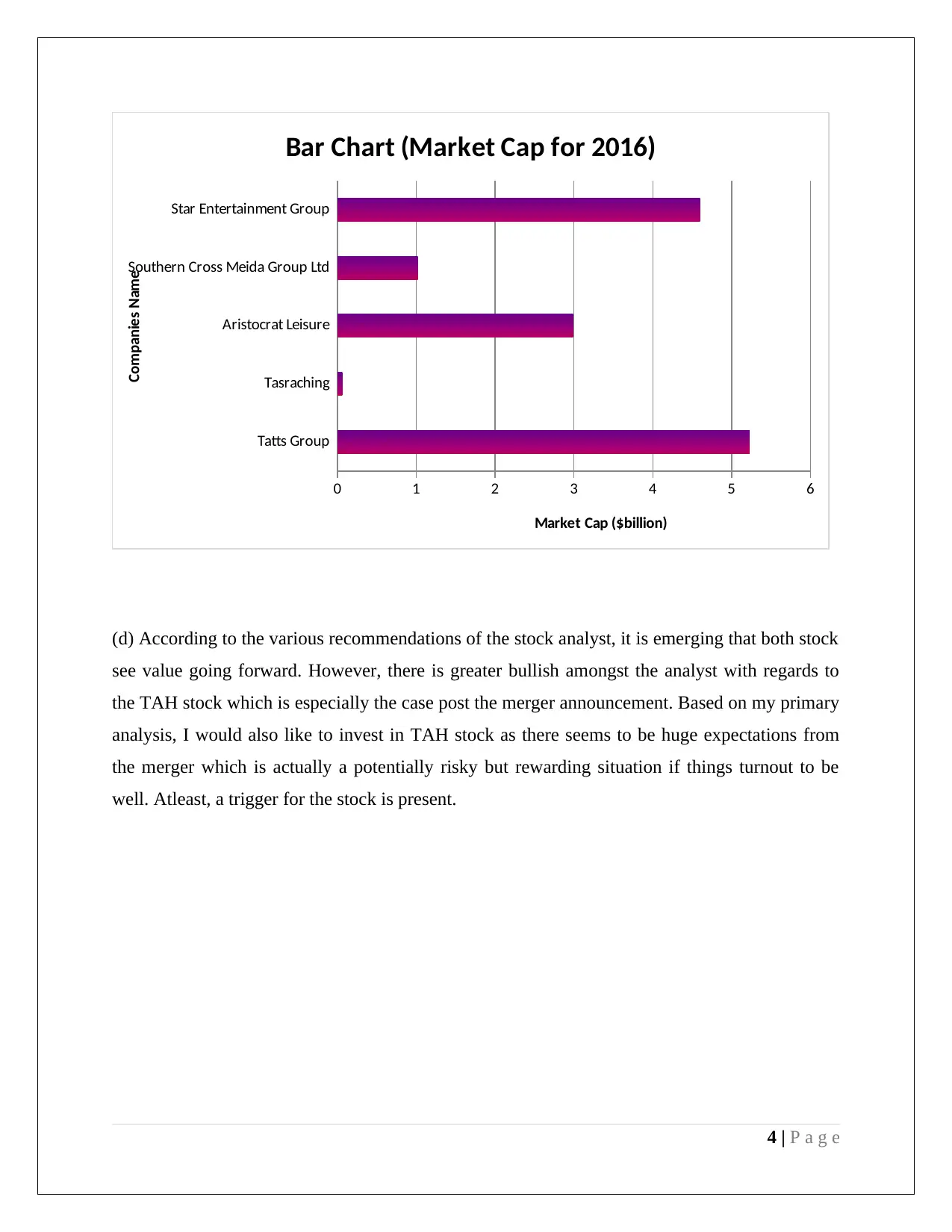
(c) The value of market capitalization for the five companies listed in ASX is highlighted
below:
3 | P a g e
below:
3 | P a g e
Secure Best Marks with AI Grader
Need help grading? Try our AI Grader for instant feedback on your assignments.
Tatts Group
Tasraching
Aristocrat Leisure
Southern Cross Meida Group Ltd
Star Entertainment Group
0 1 2 3 4 5 6
Bar Chart (Market Cap for 2016)
Market Cap ($billion)
Companies Name
(d) According to the various recommendations of the stock analyst, it is emerging that both stock
see value going forward. However, there is greater bullish amongst the analyst with regards to
the TAH stock which is especially the case post the merger announcement. Based on my primary
analysis, I would also like to invest in TAH stock as there seems to be huge expectations from
the merger which is actually a potentially risky but rewarding situation if things turnout to be
well. Atleast, a trigger for the stock is present.
4 | P a g e
Question 2
Data
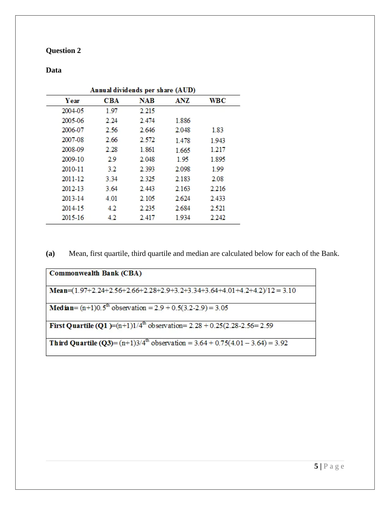
(a) Mean, first quartile, third quartile and median are calculated below for each of the Bank.
5 | P a g e
Data
(a) Mean, first quartile, third quartile and median are calculated below for each of the Bank.
5 | P a g e
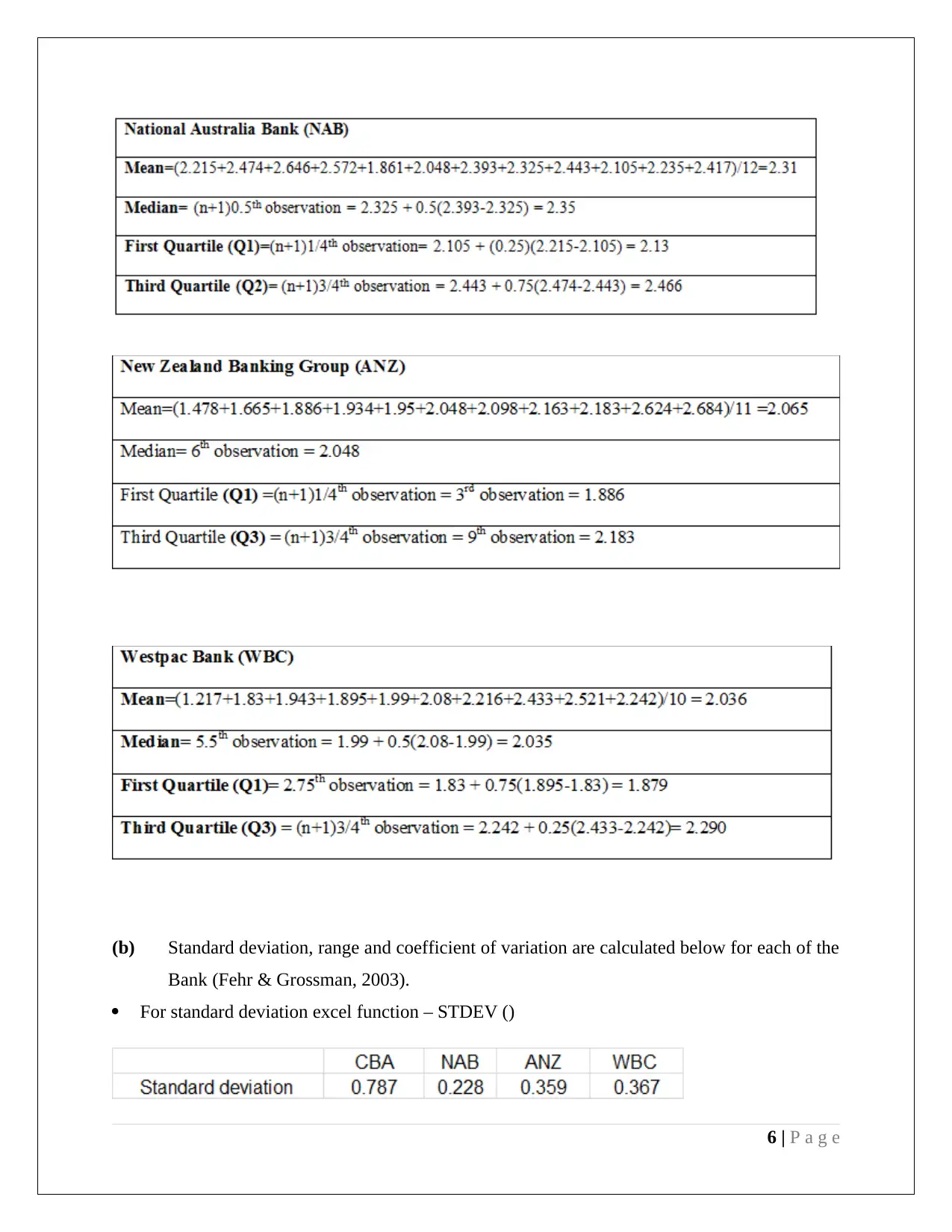
(b) Standard deviation, range and coefficient of variation are calculated below for each of the
Bank (Fehr & Grossman, 2003).
For standard deviation excel function – STDEV ()
6 | P a g e
Bank (Fehr & Grossman, 2003).
For standard deviation excel function – STDEV ()
6 | P a g e
Paraphrase This Document
Need a fresh take? Get an instant paraphrase of this document with our AI Paraphraser
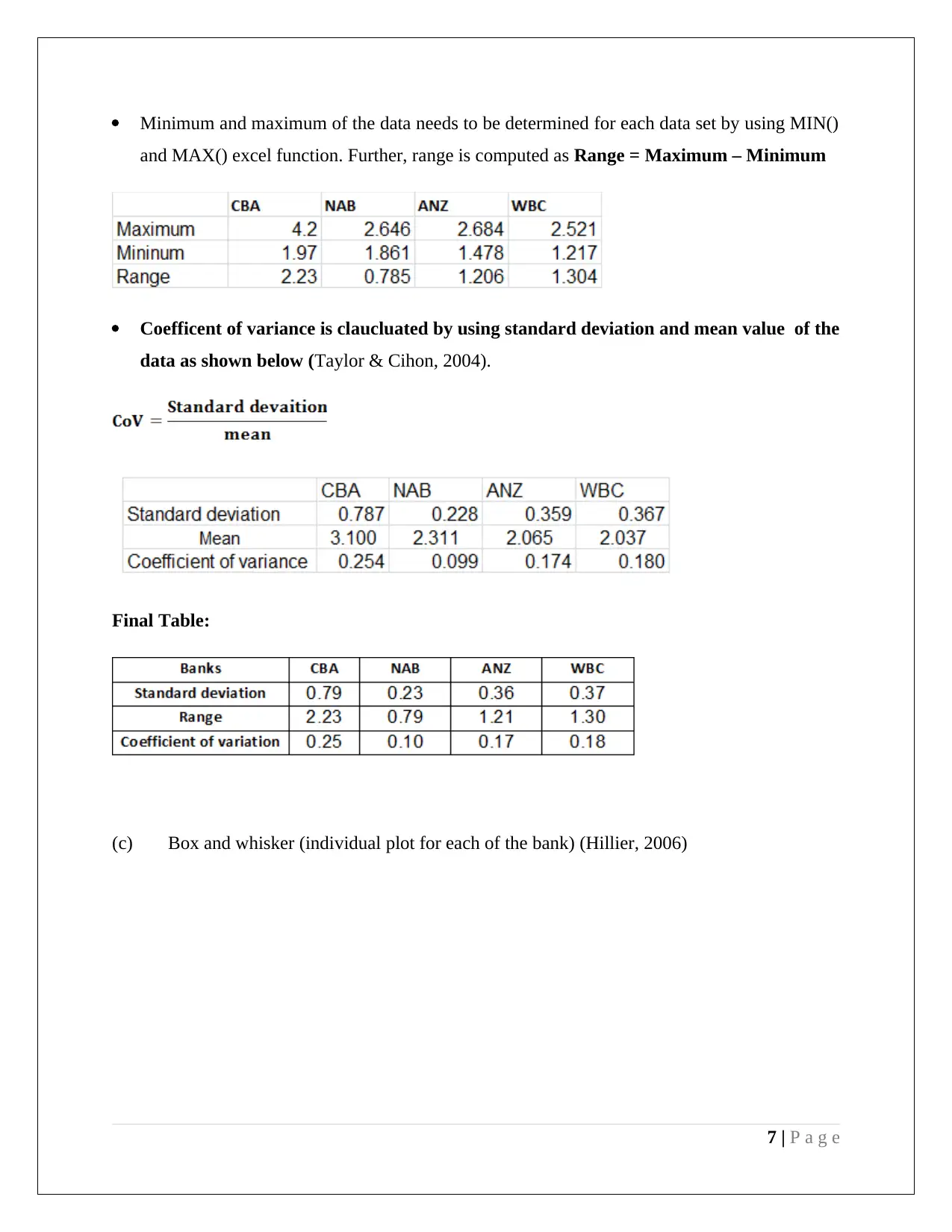
Minimum and maximum of the data needs to be determined for each data set by using MIN()
and MAX() excel function. Further, range is computed as Range = Maximum – Minimum
Coefficent of variance is claucluated by using standard deviation and mean value of the
data as shown below (Taylor & Cihon, 2004).
Final Table:
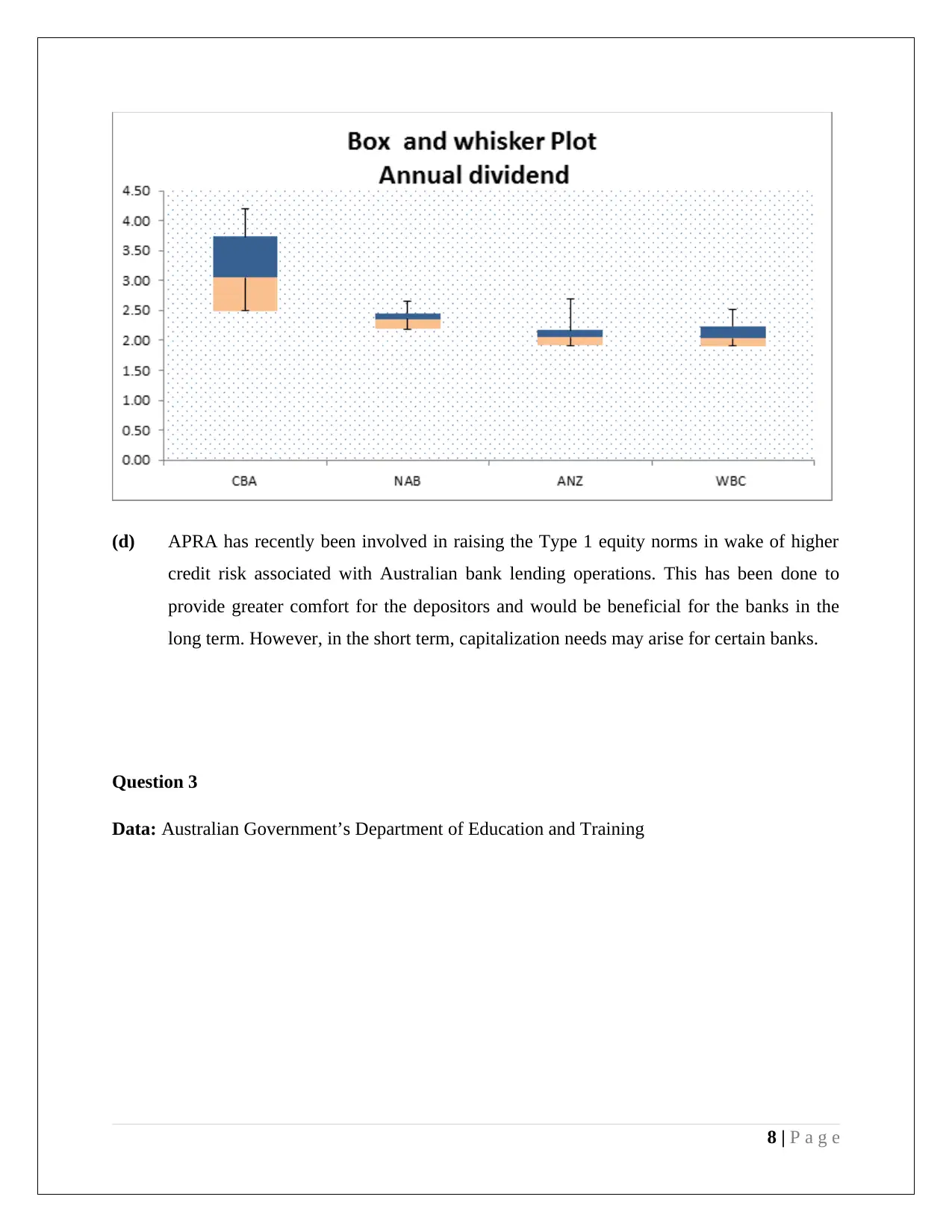
(c) Box and whisker (individual plot for each of the bank) (Hillier, 2006)
7 | P a g e
(d) APRA has recently been involved in raising the Type 1 equity norms in wake of higher
credit risk associated with Australian bank lending operations. This has been done to
provide greater comfort for the depositors and would be beneficial for the banks in the
long term. However, in the short term, capitalization needs may arise for certain banks.
Question 3
Data: Australian Government’s Department of Education and Training
8 | P a g e
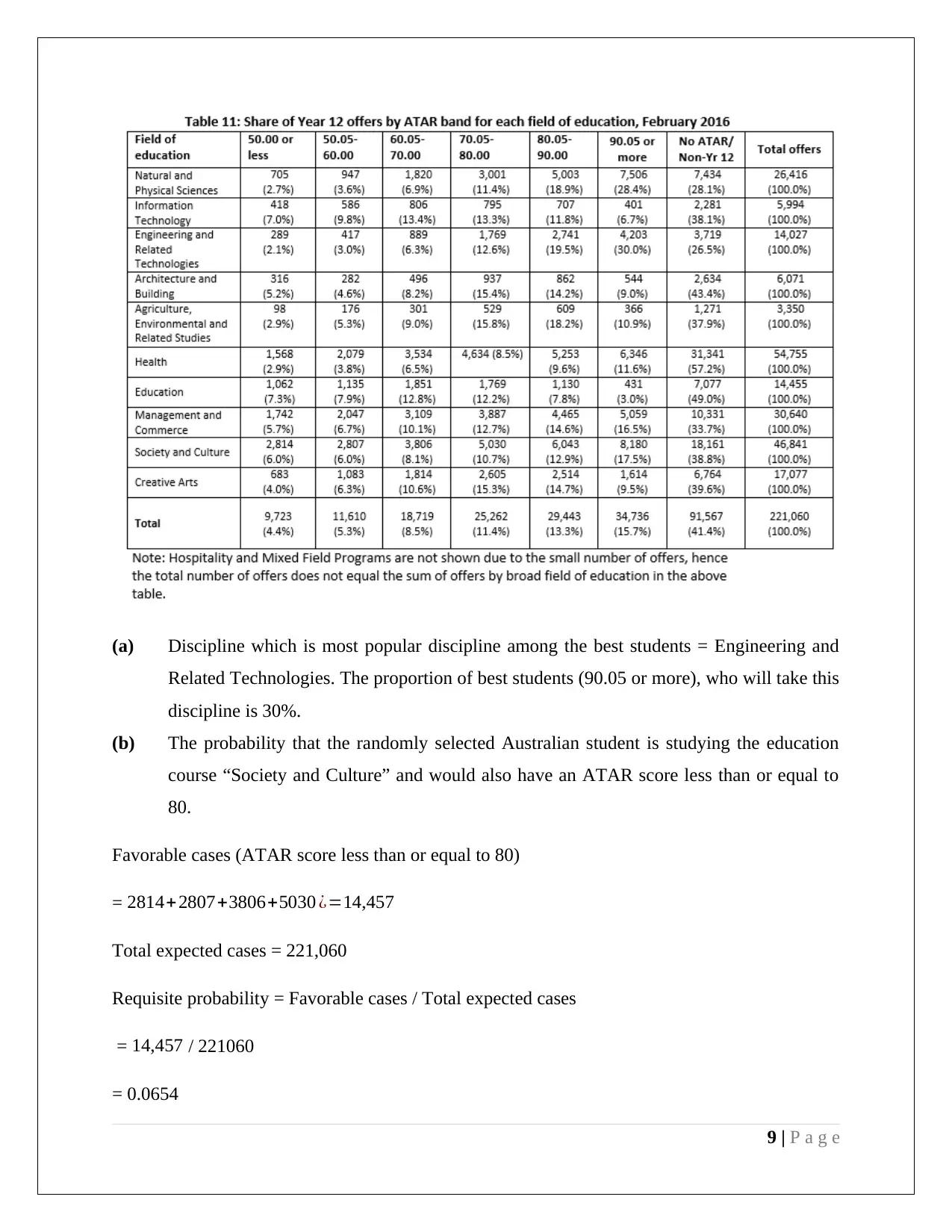
(a) Discipline which is most popular discipline among the best students = Engineering and
Related Technologies. The proportion of best students (90.05 or more), who will take this
discipline is 30%.
(b) The probability that the randomly selected Australian student is studying the education
course “Society and Culture” and would also have an ATAR score less than or equal to
80.
Favorable cases (ATAR score less than or equal to 80)
= 2814+2807+3806+5030 ¿=14,457
Total expected cases = 221,060
Requisite probability = Favorable cases / Total expected cases
= 14,457 / 221060
= 0.0654
9 | P a g e
Secure Best Marks with AI Grader
Need help grading? Try our AI Grader for instant feedback on your assignments.
Hence, there is 6.54% probability that a randomly selected Australian student is having ATAR
score less than or same as 80 and is studying society and culture.
(c) It can be seen from the data table that “Education” discipline is showing highest
proportion of the Australian students who has least ATAR grades. The proportion of
students in Education discipline with lowest ATAR score (50 or less) is 7.30%.
(d) “Health” is the discipline which shows greatest proportion of students with NO ATAR or
Non-Yr 12. A high share may be attributed to the differing interest from studies for these
students. This may make health a more compatible career path as compared to the other
fields which are more theoretical and academic.
Question 4
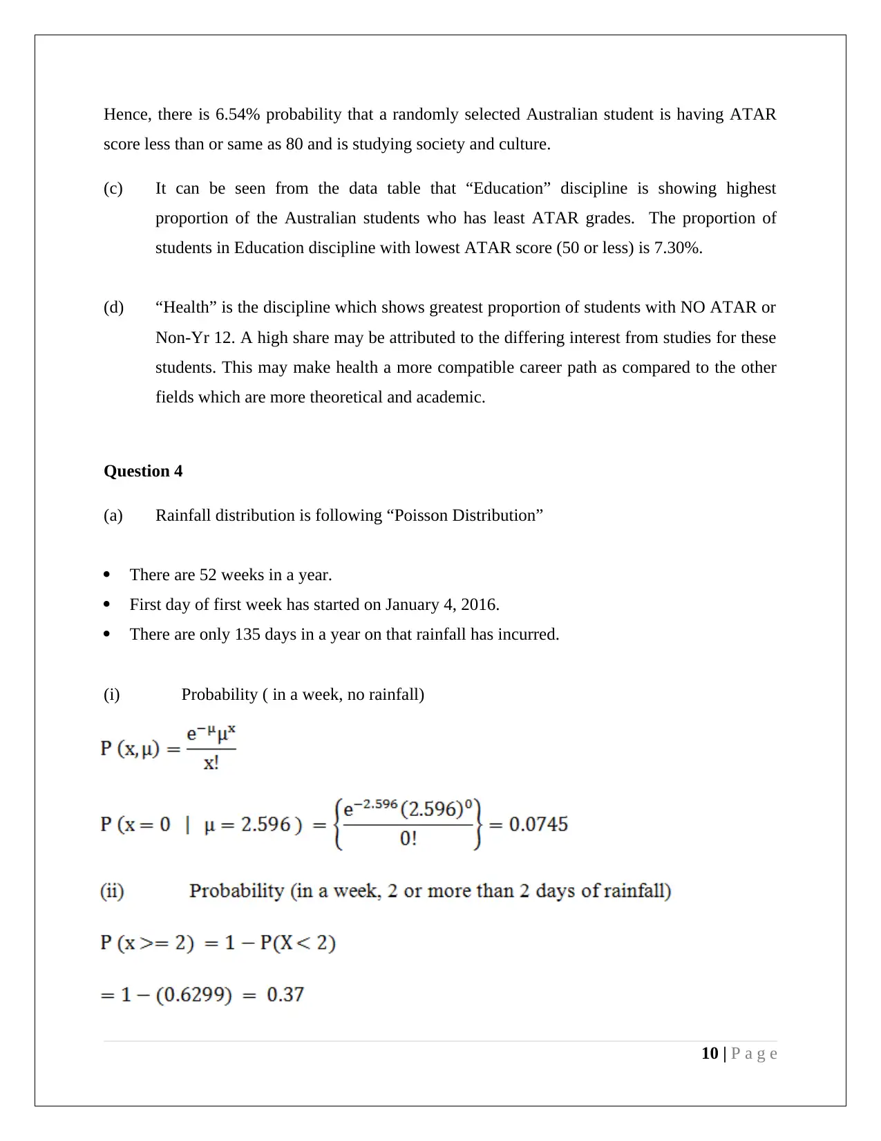
(a) Rainfall distribution is following “Poisson Distribution”
There are 52 weeks in a year.
First day of first week has started on January 4, 2016.
There are only 135 days in a year on that rainfall has incurred.
(i) Probability ( in a week, no rainfall)
10 | P a g e
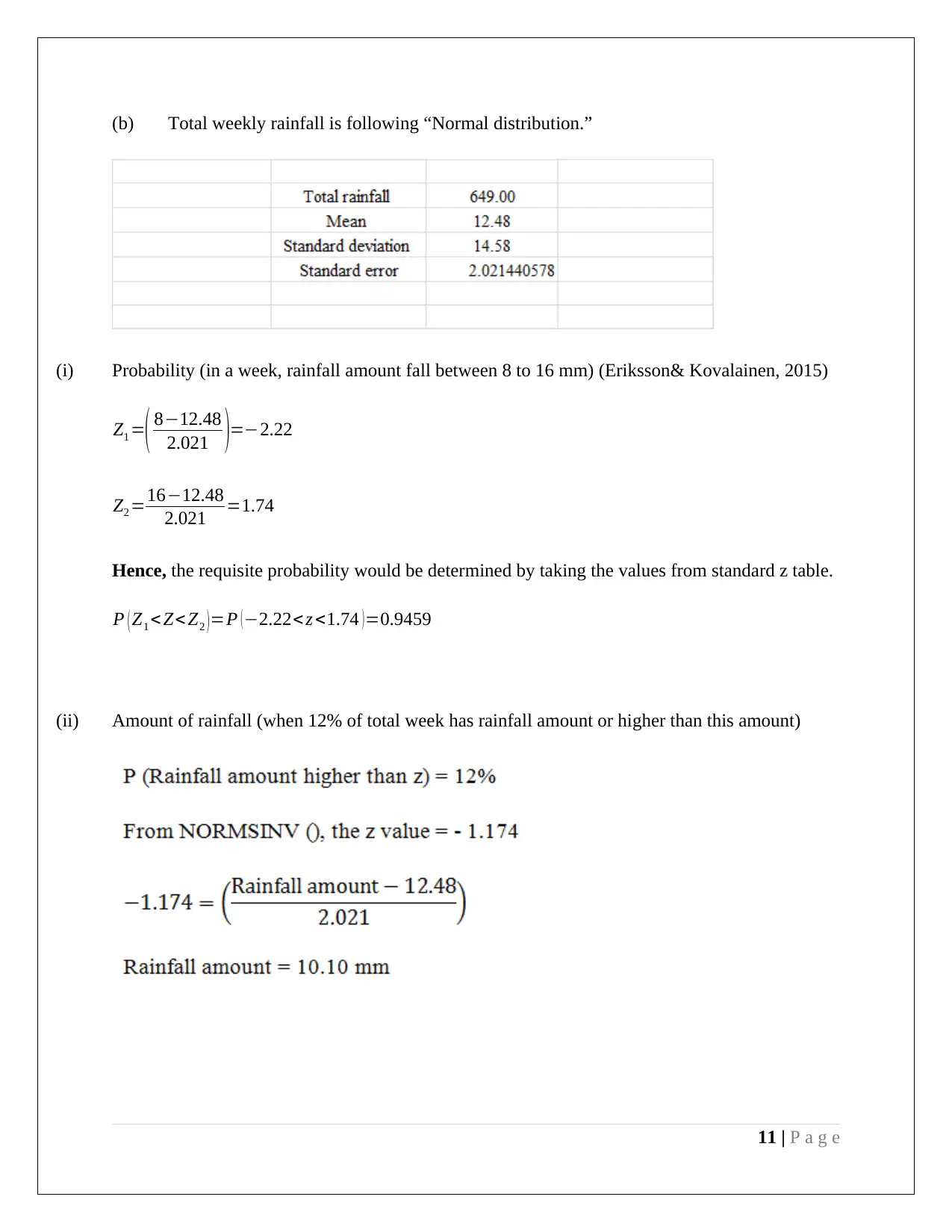
(b) Total weekly rainfall is following “Normal distribution.”
(i) Probability (in a week, rainfall amount fall between 8 to 16 mm) (Eriksson& Kovalainen, 2015)
Z1 =( 8−12.48
2.021 )=−2.22
Z2 =16−12.48
2.021 =1.74
Hence, the requisite probability would be determined by taking the values from standard z table.
P ( Z1 < Z< Z2 ) =P ( −2.22< z <1.74 ) =0.9459
(ii) Amount of rainfall (when 12% of total week has rainfall amount or higher than this amount)
11 | P a g e
Question 5
(a) Normal probability plots (Lieberman, 2013)
Interpretation: The normality is confirmed considering the above normality plots. While the
presence of outliers indicates that the variables are not perfectly normal as some skew is
present but an approximate normal distribution can be assumed.
(b) 95% confidence interval has been determined by using KADD add in of excel. The output
are showing below (Flick, 2015).
12 | P a g e
Paraphrase This Document
Need a fresh take? Get an instant paraphrase of this document with our AI Paraphraser
13 | P a g e
(c) Hypothesis testing (Shi & Tao, 2008)
14 | P a g e
14 | P a g e
The p value approach is used. As significance level is lesser than p value, hence null hypothesis
rejection cannot happen. It leads to conclusion that difference between this variable for bankrupt
and non-bankrupt firms does not seem significant from a statistical standpoint.
The p value approach is used. As significance level is greater than p value, hence null hypothesis
rejection would happen. It leads to conclusion that difference between this variable for bankrupt
and non-bankrupt firms does seem significant from a statistical standpoint.
15 | P a g e
Secure Best Marks with AI Grader
Need help grading? Try our AI Grader for instant feedback on your assignments.
The p value approach is used. As significance level is greater than p value, hence null hypothesis
rejection would happen. It leads to conclusion that difference between this variable for bankrupt
and non-bankrupt firms does seem significant from a statistical standpoint.
The p value approach is used. As significance level is greater than p value, hence null hypothesis
rejection would happen. It leads to conclusion that difference between this variable for bankrupt
and non-bankrupt firms does seem significant from a statistical standpoint.
16 | P a g e
rejection would happen. It leads to conclusion that difference between this variable for bankrupt
and non-bankrupt firms does seem significant from a statistical standpoint.
The p value approach is used. As significance level is greater than p value, hence null hypothesis
rejection would happen. It leads to conclusion that difference between this variable for bankrupt
and non-bankrupt firms does seem significant from a statistical standpoint.
16 | P a g e
The p value approach is used. As significance level is greater than p value, hence null hypothesis
rejection would happen. It leads to conclusion that difference between this variable for bankrupt
and non-bankrupt firms does seem significant from a statistical standpoint.
The p value approach is used. As significance level is lesser than p value, hence null hypothesis
rejection cannot happen. It leads to conclusion that difference between this variable for bankrupt
and non-bankrupt firms does not seem significant from a statistical standpoint.
17 | P a g e
Reference
Eriksson, P. & Kovalainen, A. (2015). Quantitative methods in business research (3rd ed.).
London: Sage Publications.
Fehr, F. H., & Grossman, G. (2003). An introduction to sets, probability and hypothesis testing
(3rd ed.). Ohio: Heath.
Flick, U. (2015). Introducing research methodology: A beginner's guide to doing a research
project (4th ed.). New York: Sage Publications.
Hillier, F. (2006). Introduction to Operations Research. (6th ed.). New York: McGraw Hill
Publications.
Lieberman, F. J., Nag, B., Hiller, F.S. & Basu, P. (2013). Introduction To Operations Research
(5th ed.). New Delhi: Tata McGraw Hill Publishers.
Shi, Z. N. & Tao, J. (2008). Statistical Hypothesis Testing: Theory and Methods (6th ed.).
London: World Scientific.
Taylor, K. J. & Cihon, C. (2004). Statistical Techniques for Data Analysis (2nd ed.). Melbourne:
CRC Press.
18 | P a g e
Paraphrase This Document
Need a fresh take? Get an instant paraphrase of this document with our AI Paraphraser
19 | P a g e
1 out of 20
Related Documents
Your All-in-One AI-Powered Toolkit for Academic Success.
+13062052269
info@desklib.com
Available 24*7 on WhatsApp / Email
Unlock your academic potential
© 2024 | Zucol Services PVT LTD | All rights reserved.