Statistics for Market Price and Age of House

This report provides detailed statistics for market price and age of house including summary statistics, scatter plot, multiple regression model, and correlation. It also covers the selection of random sampling and interpretation of results. The sample size for the present study is 50 and the independent variables include Sydney price Index, Total number of square meters, and Age of house (years).

Statistics

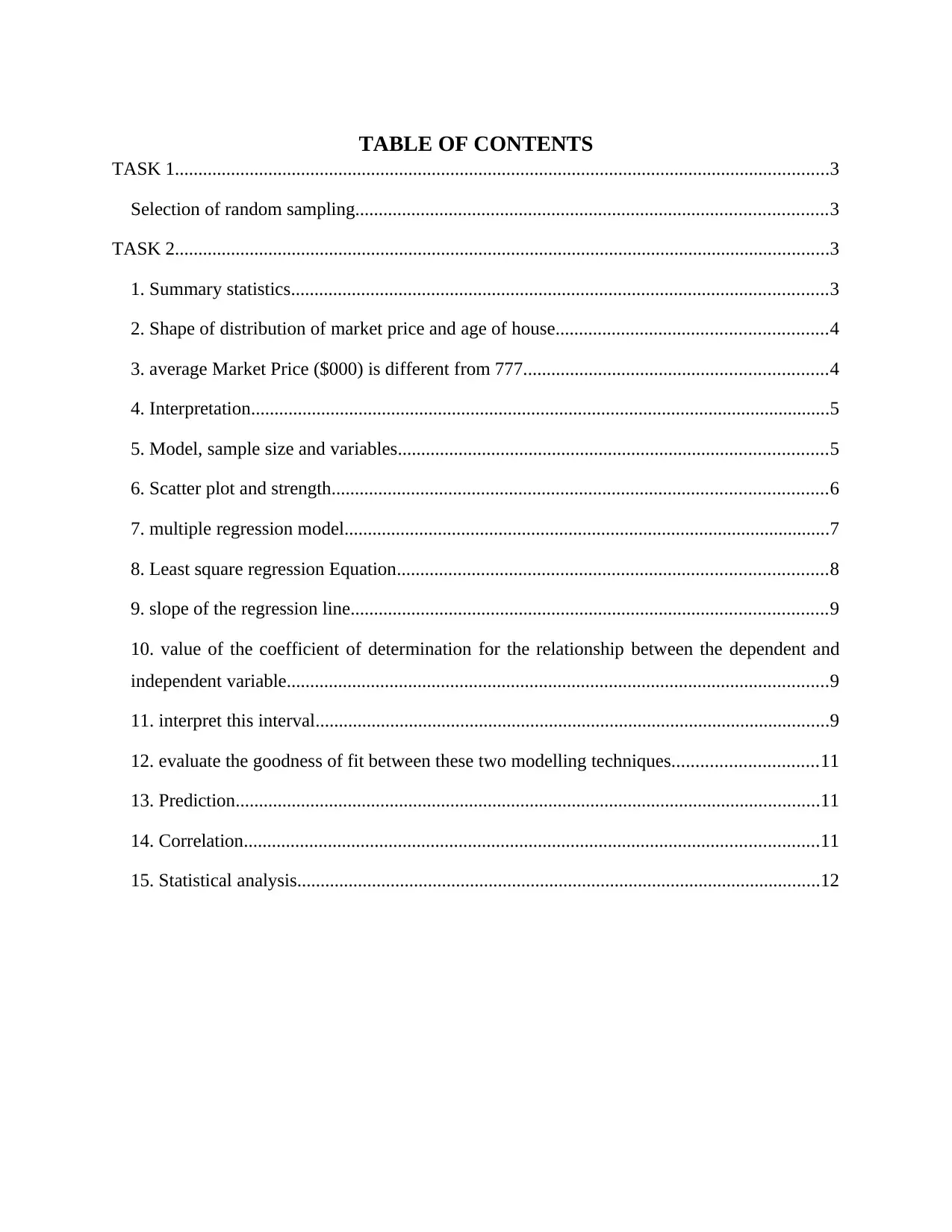
TABLE OF CONTENTS
TASK 1............................................................................................................................................3
Selection of random sampling.....................................................................................................3
TASK 2............................................................................................................................................3
1. Summary statistics...................................................................................................................3
2. Shape of distribution of market price and age of house..........................................................4
3. average Market Price ($000) is different from 777.................................................................4
4. Interpretation............................................................................................................................5
5. Model, sample size and variables............................................................................................5
6. Scatter plot and strength..........................................................................................................6
7. multiple regression model........................................................................................................7
8. Least square regression Equation............................................................................................8
9. slope of the regression line......................................................................................................9
10. value of the coefficient of determination for the relationship between the dependent and
independent variable....................................................................................................................9
11. interpret this interval..............................................................................................................9
12. evaluate the goodness of fit between these two modelling techniques...............................11
13. Prediction.............................................................................................................................11
14. Correlation...........................................................................................................................11
15. Statistical analysis................................................................................................................12

TASK 1
Selection of random sampling
Enclosed in Excel
TASK 2
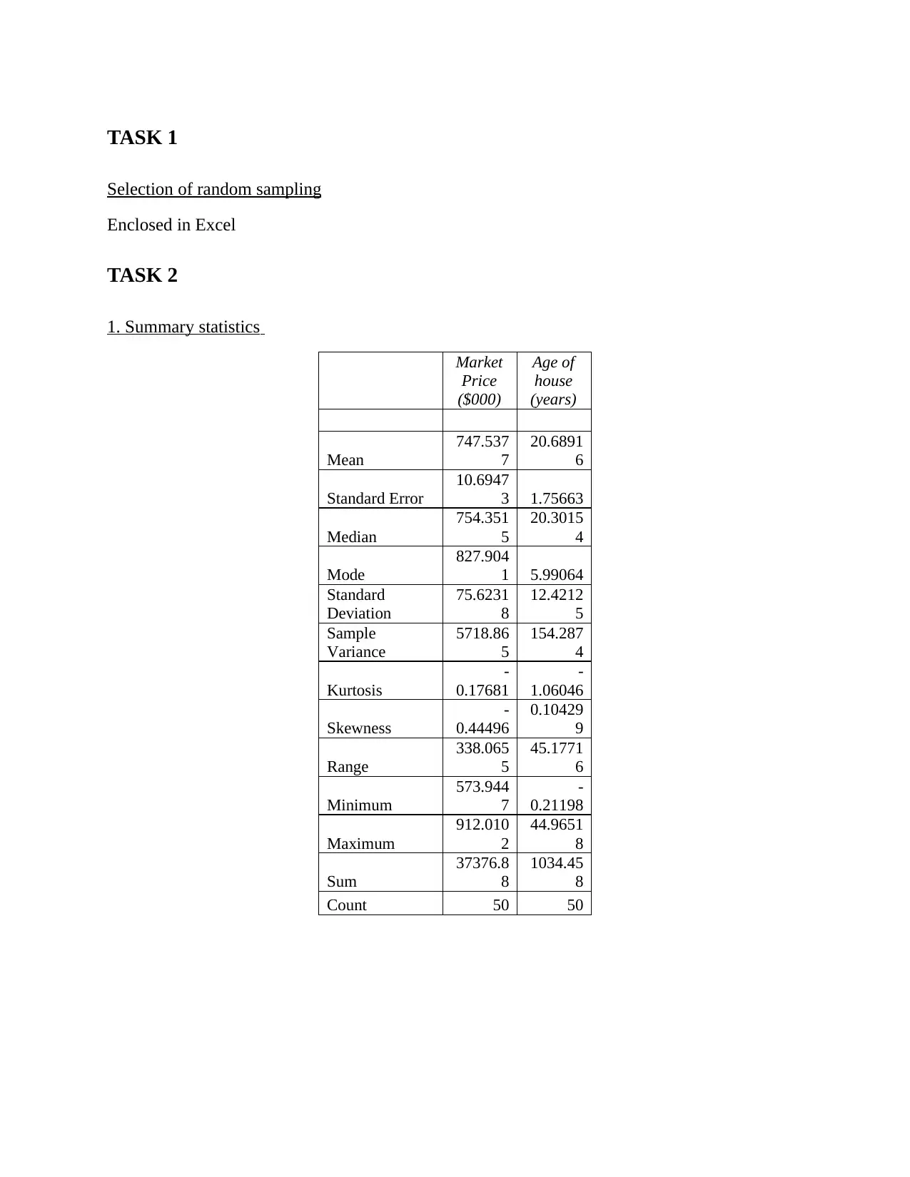
1. Summary statistics
Market
Price
($000)
Age of
house
(years)
Mean
747.537
7
20.6891
6
Standard Error
10.6947
3 1.75663
Median
754.351
5
20.3015
4
Mode
827.904
1 5.99064
Standard
Deviation
75.6231
8
12.4212
5
Sample
Variance
5718.86
5
154.287
4
Kurtosis
-
0.17681
-
1.06046
Skewness
-
0.44496
0.10429
9
Range
338.065
5
45.1771
6
Minimum
573.944
7
-
0.21198
Maximum
912.010
2
44.9651
8
Sum
37376.8
8
1034.45
8
Count 50 50

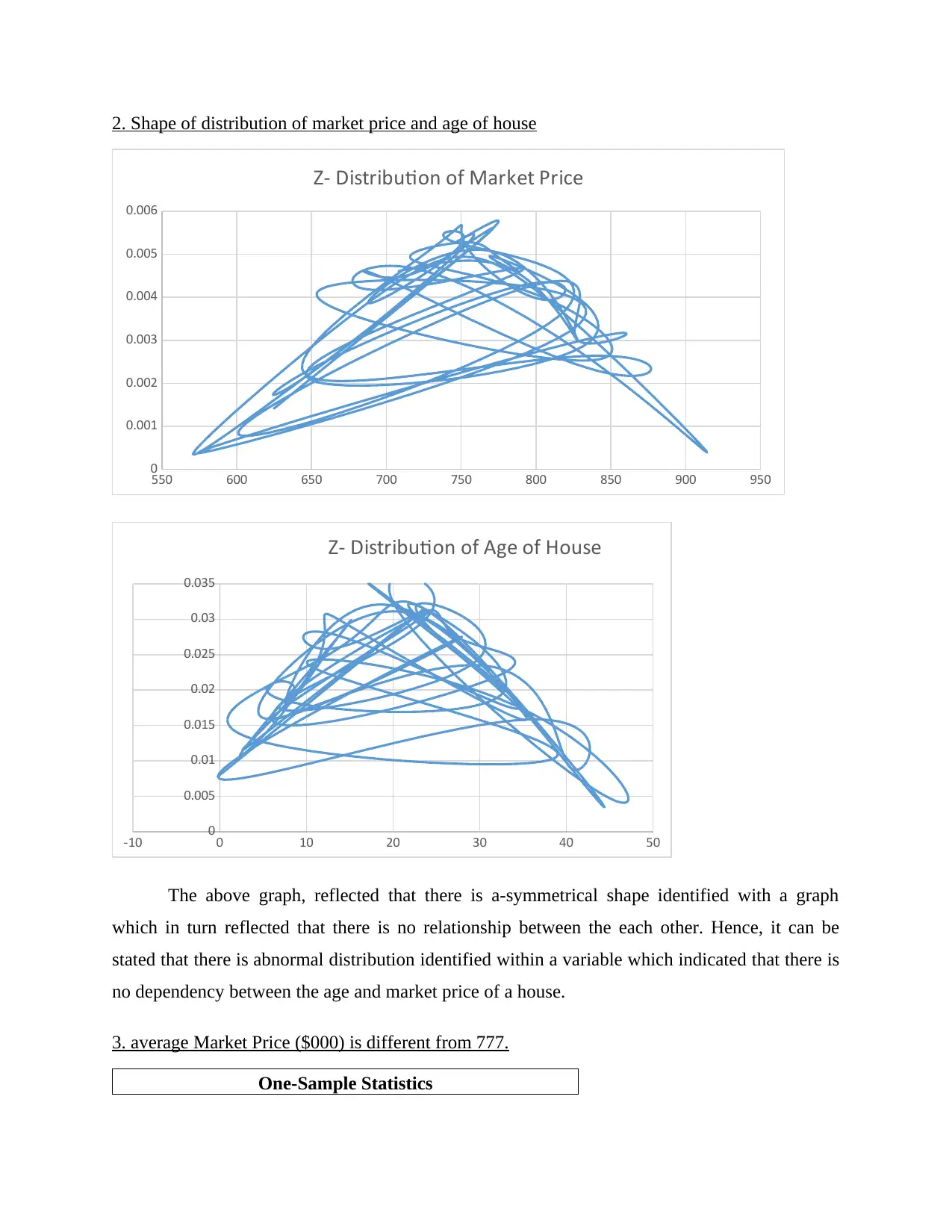
2. Shape of distribution of market price and age of house
550 600 650 700 750 800 850 900 950
0
0.001
0.002
0.003
0.004
0.005
0.006
Z- Distribution of Market Price
-10 0 10 20 30 40 50
0
0.005
0.01
0.015
0.02
0.025
0.03
0.035
Z- Distribution of Age of House
The above graph, reflected that there is a-symmetrical shape identified with a graph
which in turn reflected that there is no relationship between the each other. Hence, it can be
stated that there is abnormal distribution identified within a variable which indicated that there is
no dependency between the age and market price of a house.
3. average Market Price ($000) is different from 777.
One-Sample Statistics

N Mean Std.
Deviation
Std. Error
Mean
market 400 777.04 79.385 3.969
One-Sample Test
Test Value = 777
t df Sig. (2-
tailed)
Mean
Difference
95% Confidence Interval of
the Difference
Lower Upper
market .009 399 .992 .038 -7.77 7.84
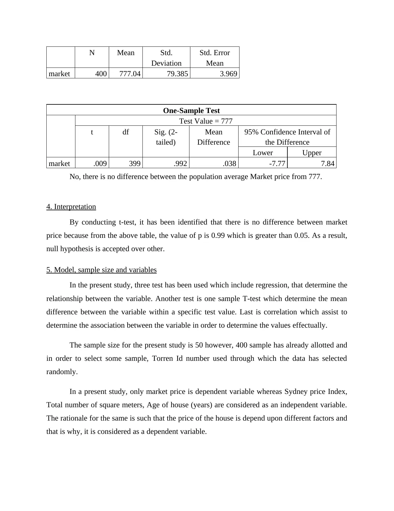
No, there is no difference between the population average Market price from 777.
4. Interpretation
By conducting t-test, it has been identified that there is no difference between market
price because from the above table, the value of p is 0.99 which is greater than 0.05. As a result,
null hypothesis is accepted over other.
5. Model, sample size and variables
In the present study, three test has been used which include regression, that determine the
relationship between the variable. Another test is one sample T-test which determine the mean
difference between the variable within a specific test value. Last is correlation which assist to
determine the association between the variable in order to determine the values effectually.
The sample size for the present study is 50 however, 400 sample has already allotted and
in order to select some sample, Torren Id number used through which the data has selected
randomly.
In a present study, only market price is dependent variable whereas Sydney price Index,
Total number of square meters, Age of house (years) are considered as an independent variable.
The rationale for the same is such that the price of the house is depend upon different factors and
that is why, it is considered as a dependent variable.

6. Scatter plot and strength
0.0
100.0
200.0
300.0
400.0
0
500
1000
Total number of square
meters Line Fit Plot
Market Price ($000)
Predicted Market
Price ($000)
Linear (Predicted
Market Price ($000))
Total number of square meters
Market Price ($000)
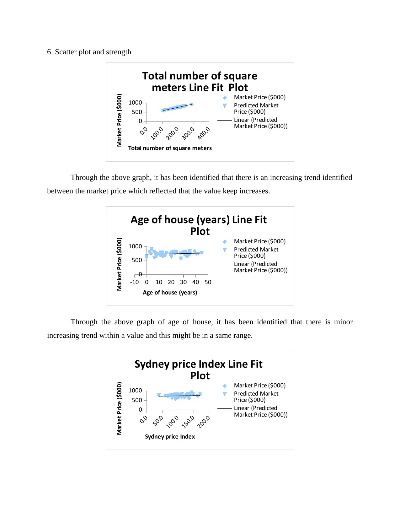
Through the above graph, it has been identified that there is an increasing trend identified
between the market price which reflected that the value keep increases.
-10 0 10 20 30 40 50
0
500
1000
Age of house (years) Line Fit
Plot Market Price ($000)
Predicted Market
Price ($000)
Linear (Predicted
Market Price ($000))
Age of house (years)
Market Price ($000)
Through the above graph of age of house, it has been identified that there is minor
increasing trend within a value and this might be in a same range.
0.0
50.0
100.0
150.0
200.0
0
500
1000
Sydney price Index Line Fit
Plot Market Price ($000)
Predicted Market
Price ($000)
Linear (Predicted
Market Price ($000))
Sydney price Index
Market Price ($000)

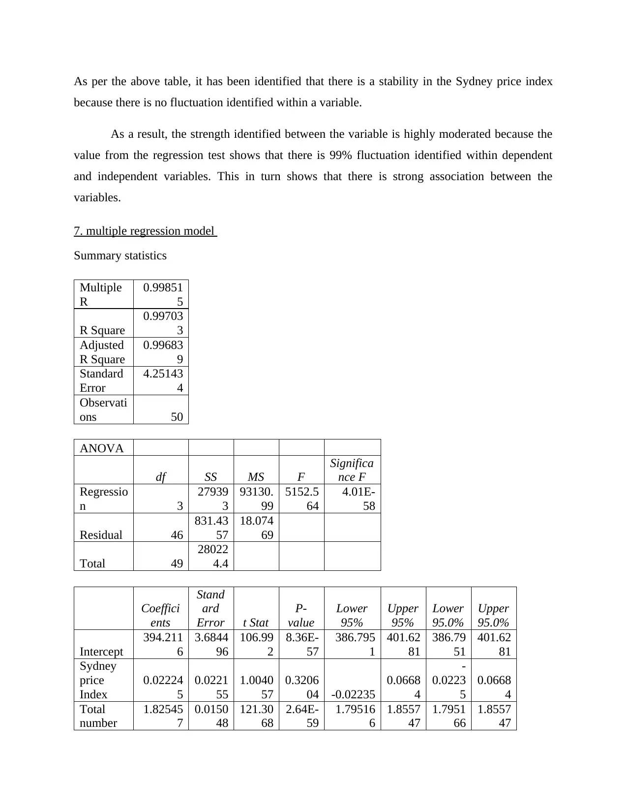
As per the above table, it has been identified that there is a stability in the Sydney price index
because there is no fluctuation identified within a variable.
As a result, the strength identified between the variable is highly moderated because the
value from the regression test shows that there is 99% fluctuation identified within dependent
and independent variables. This in turn shows that there is strong association between the
variables.
7. multiple regression model
Summary statistics
Multiple
R
0.99851
5
R Square
0.99703
3
Adjusted
R Square
0.99683
9
Standard
Error
4.25143
4
Observati
ons 50
ANOVA
df SS MS F
Significa
nce F
Regressio
n 3
27939
3
93130.
99
5152.5
64
4.01E-
58
Residual 46
831.43
57
18.074
69
Total 49
28022
4.4
Coeffici
ents
Stand
ard
Error t Stat
P-
value
Lower
95%
Upper
95%
Lower
95.0%
Upper
95.0%
Intercept
394.211
6
3.6844
96
106.99
2
8.36E-
57
386.795
1
401.62
81
386.79
51
401.62
81
Sydney
price
Index
0.02224
5
0.0221
55
1.0040
57
0.3206
04 -0.02235
0.0668
4
-
0.0223
5
0.0668
4
Total
number
1.82545
7
0.0150
48
121.30
68
2.64E-
59
1.79516
6
1.8557
47
1.7951
66
1.8557
47

of square
meters
Age of
house
(years)
-
0.03613
0.0508
18
-
0.7108
8
0.4807
46 -0.13842
0.0661
66
-
0.1384
2
0.0661
66
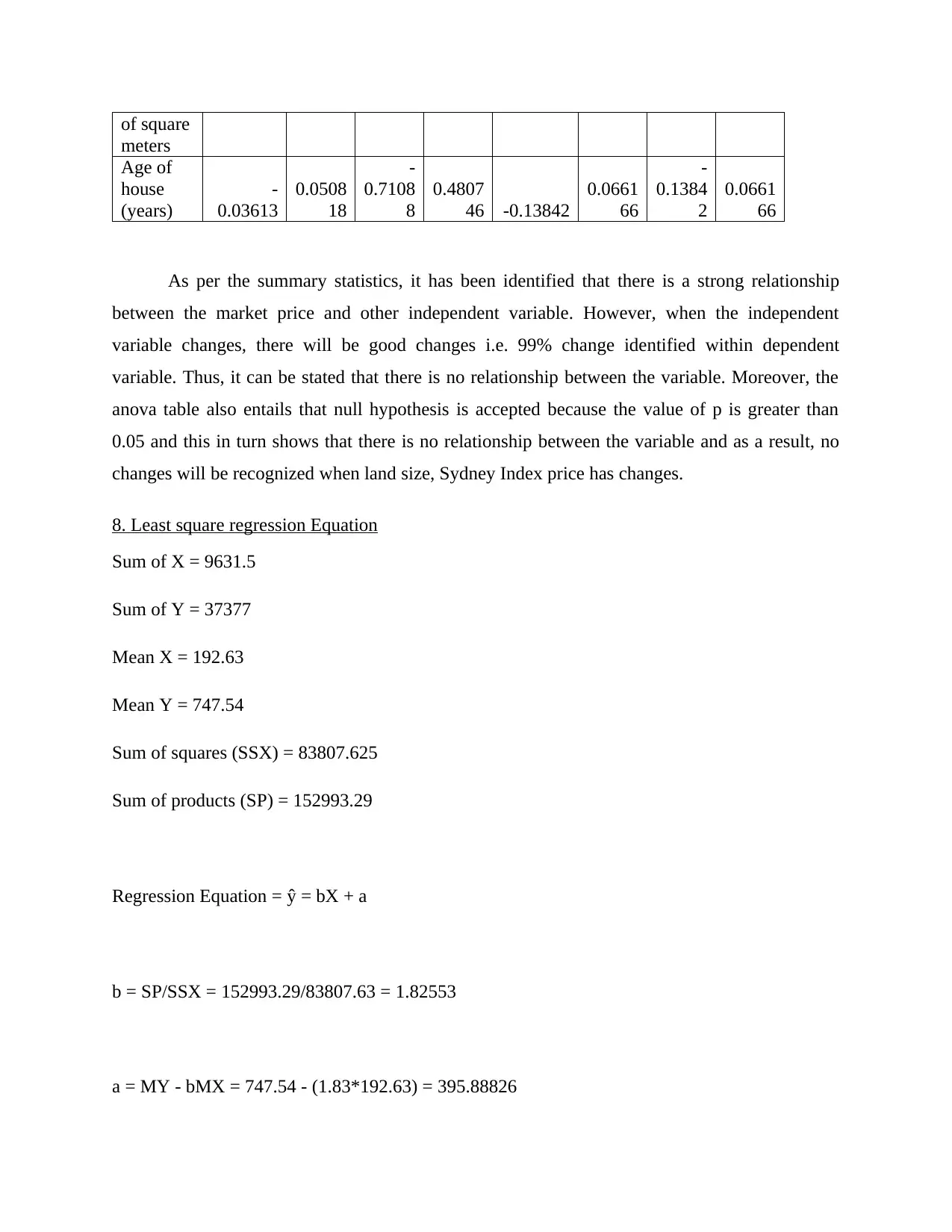
As per the summary statistics, it has been identified that there is a strong relationship
between the market price and other independent variable. However, when the independent
variable changes, there will be good changes i.e. 99% change identified within dependent
variable. Thus, it can be stated that there is no relationship between the variable. Moreover, the
anova table also entails that null hypothesis is accepted because the value of p is greater than
0.05 and this in turn shows that there is no relationship between the variable and as a result, no
changes will be recognized when land size, Sydney Index price has changes.
8. Least square regression Equation
Sum of X = 9631.5
Sum of Y = 37377
Mean X = 192.63
Mean Y = 747.54
Sum of squares (SSX) = 83807.625
Sum of products (SP) = 152993.29
Regression Equation = ŷ = bX + a
b = SP/SSX = 152993.29/83807.63 = 1.82553
a = MY - bMX = 747.54 - (1.83*192.63) = 395.88826

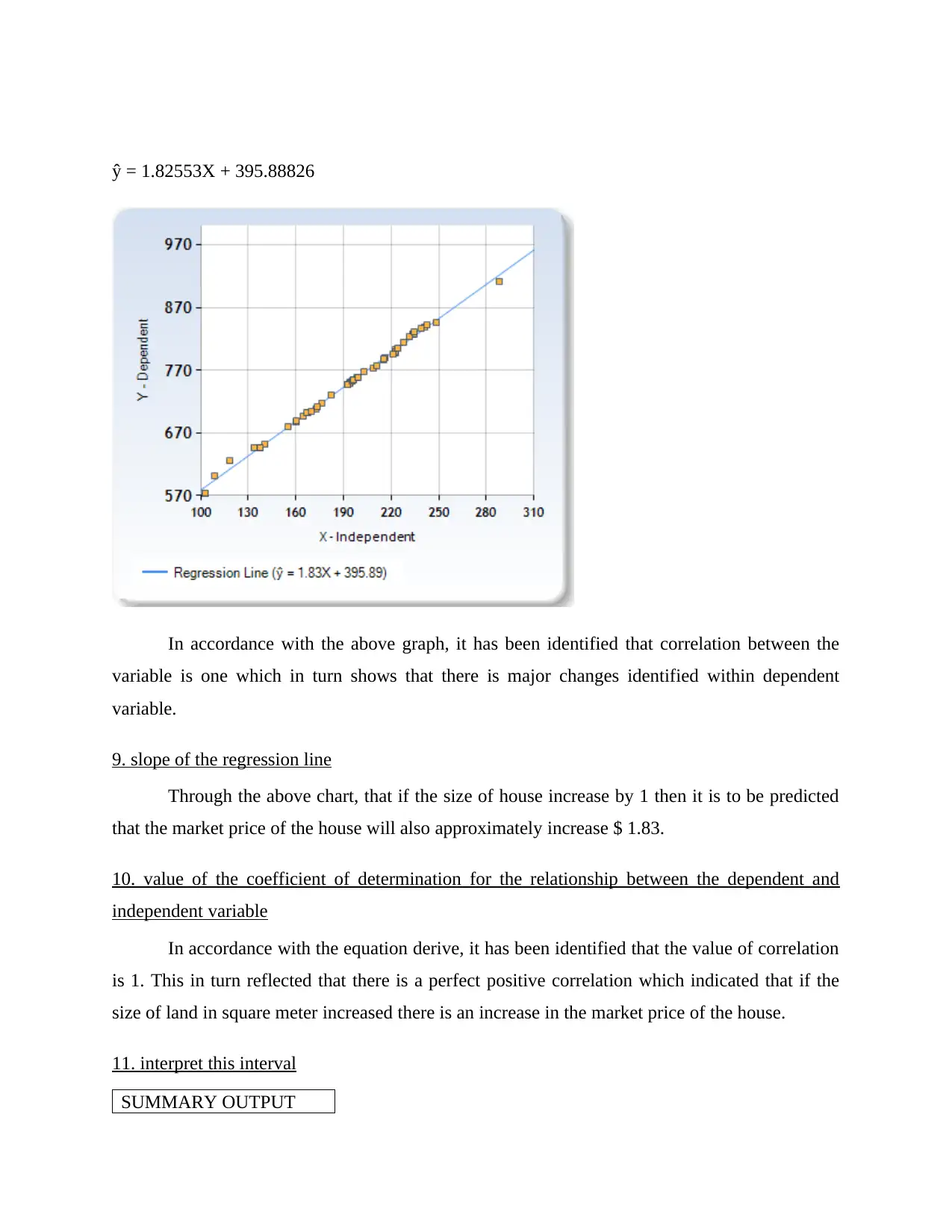
ŷ = 1.82553X + 395.88826
In accordance with the above graph, it has been identified that correlation between the
variable is one which in turn shows that there is major changes identified within dependent
variable.
9. slope of the regression line
Through the above chart, that if the size of house increase by 1 then it is to be predicted
that the market price of the house will also approximately increase $ 1.83.
10. value of the coefficient of determination for the relationship between the dependent and
independent variable
In accordance with the equation derive, it has been identified that the value of correlation
is 1. This in turn reflected that there is a perfect positive correlation which indicated that if the
size of land in square meter increased there is an increase in the market price of the house.
11. interpret this interval
SUMMARY OUTPUT

Regression Statistics
Multiple R
0.9984
52
R Square
0.9969
07
Adjusted R
Square
0.9968
42
Standard Error
4.2495
61
Observations 50
ANOVA
df SS MS F
Signific
ance F
Regression 1
279357.
6
2793
57.6
1546
9.36
6.76E-
62
Residual 48
866.820
9
18.0
5877
Total 49
280224.
4
Coeffi
cients
Standar
d Error t Stat
P-
valu
e
Lower
95%
Upper
95%
Lower
95.0%
Upper
95.0%
Intercept
395.81
57 2.89105
136.
9107
6.82
E-64
390.002
8
401.62
85
390.00
28
401.62
85
Total number of
square meters
1.8259
4
0.01468
1
124.
3759
6.76
E-62
1.79642
2
1.8554
58
1.7964
22
1.8554
58
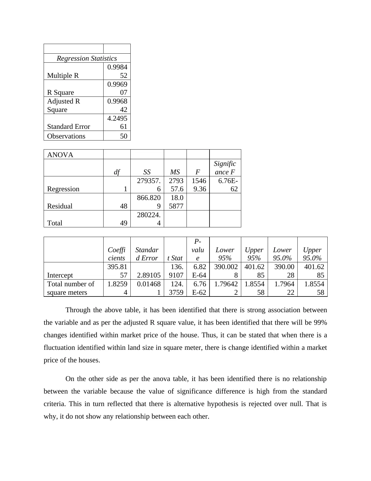
Through the above table, it has been identified that there is strong association between
the variable and as per the adjusted R square value, it has been identified that there will be 99%
changes identified within market price of the house. Thus, it can be stated that when there is a
fluctuation identified within land size in square meter, there is change identified within a market
price of the houses.
On the other side as per the anova table, it has been identified there is no relationship
between the variable because the value of significance difference is high from the standard
criteria. This in turn reflected that there is alternative hypothesis is rejected over null. That is
why, it do not show any relationship between each other.

12. evaluate the goodness of fit between these two modelling techniques.
From the simple linear regression and multiple regression model, it has been identified
that there is a no change recorded within a goodness of fit. The rationale of this is such that it
allows to evaluate the relationship between two variables by controlling the effect of other
variables. Hence, it can be stated that there is a changes identified over goodness of fit like under
multiple regression, only strong relationship identified because the value of R square is 0.99
which is fall under the category of 0.25 to 0.50. However, in simple linear regression equation,
the value is 0.99 which around 1 that depicts positive correlation between the variables.
Therefore, both the technique is good to used which help to create a better outcome and
determine the dependency between the variable.
13. Prediction
At the value of 300, the market price will be $943.59. Yes, the answer is true because the
results has generated by using a formula of forecast. This in turn assist to shows that the answer
is valid and at such a high square meter, the value of the market price will be high.
14. Correlation
Correlations
marketprice landsize
marketprice
Pearson Correlation 1 .998**
Sig. (2-tailed) .000
N 50 50
landsize
Pearson Correlation .998** 1
Sig. (2-tailed) .000
N 50 50
**. Correlation is significant at the 0.01 level (2-tailed).
In accordance with the above table, it has been identified that there is strong positive
relationship between the variable and that is why, it provide accurate results. Also, having such a
strong relationship between all the variable reflected that it predict the value in accurate manner.
Therefore, it can be stated that opting land size in order to predict the market value will be
beneficial to generate a better answer and ascertain the future value as well.

15. Statistical analysis
a)
Null hypothesis: There is no association between the market price and land size in square
meter in house.
Alternative hypothesis: There is an association between the market price and land size in
square meter in house.
b)
In accordance with the correlation table, it has been identified that the significance value
is 0.00 which is lower than the standard criteria i.e. 0.05. Therefore, it can be reflected that it will
provide accurate results and determine the market price of a house in effective manner. Hence,
alternative hypothesis is accepted over null and this shows that there will be a positive
relationship shared between the variable.
c)
As per the results generated, it has been identified that there is a strong relationship
between the variable in which it has been identified that when the value of land size within an
area will changes there will be a direct impact identified within the market price. That is why, it
will be better to predict the values in the market size so that it identified the values in appropriate
manner.