Statistics Problems: Comparing Return Data from Newbury and Dedham

This homework assignment presents a student's statistical analysis of item return data from two locations, Newbury and Dedham. The analysis includes three parts: a chi-square test to compare the proportion of NERDZERK days, an ANOVA test to assess the difference in variances of returns, and a...Read More

1
Statistics Problems
Student Name: Student ID:
Due Date: Unit Name:

2
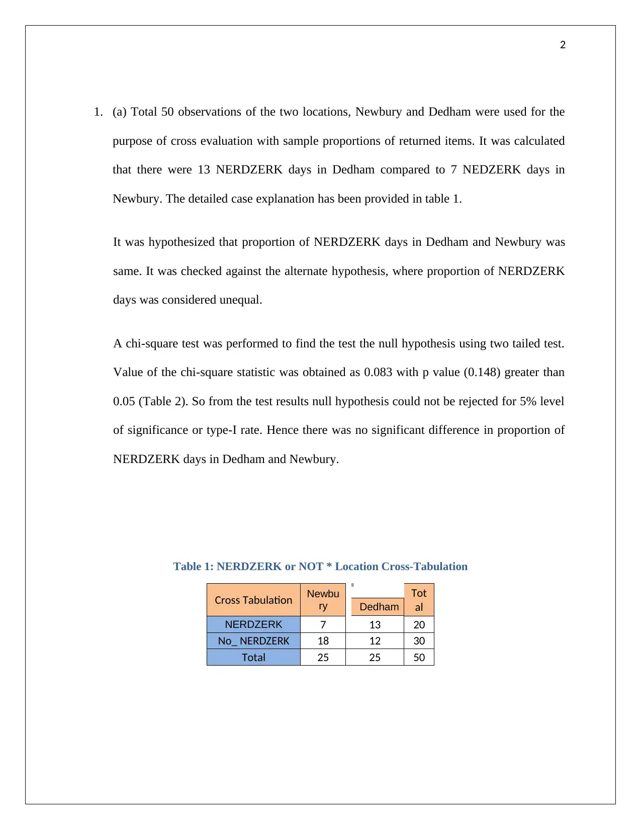
1. (a) Total 50 observations of the two locations, Newbury and Dedham were used for the
purpose of cross evaluation with sample proportions of returned items. It was calculated
that there were 13 NERDZERK days in Dedham compared to 7 NEDZERK days in
Newbury. The detailed case explanation has been provided in table 1.
It was hypothesized that proportion of NERDZERK days in Dedham and Newbury was
same. It was checked against the alternate hypothesis, where proportion of NERDZERK
days was considered unequal.
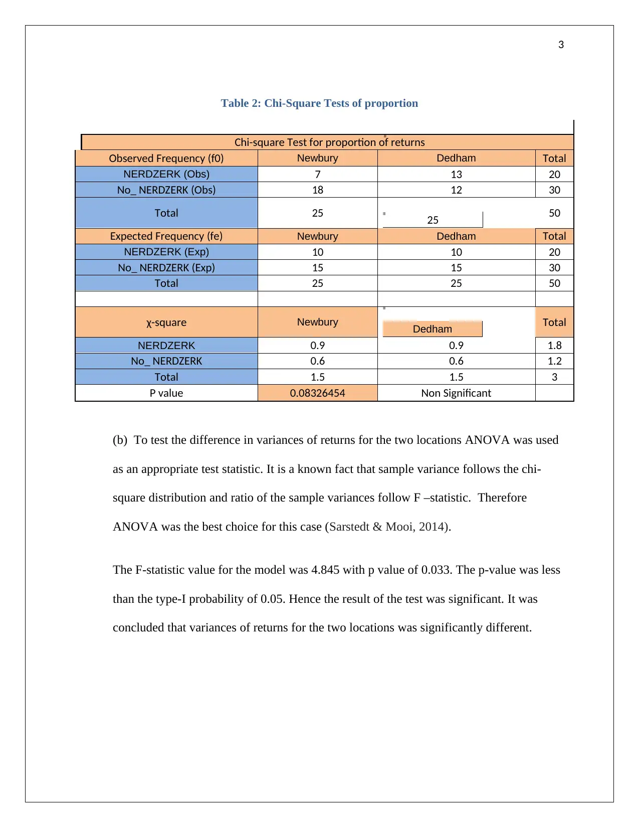
A chi-square test was performed to find the test the null hypothesis using two tailed test.
Value of the chi-square statistic was obtained as 0.083 with p value (0.148) greater than
0.05 (Table 2). So from the test results null hypothesis could not be rejected for 5% level
of significance or type-I rate. Hence there was no significant difference in proportion of
NERDZERK days in Dedham and Newbury.
Table 1: NERDZERK or NOT * Location Cross-Tabulation
Cross Tabulation Newbu
ry Dedham
Tot
al
NERDZERK 7 13 20
No_ NERDZERK 18 12 30
Total 25 25 50

3
Table 2: Chi-Square Tests of proportion
Chi-square Test for proportion of returns
Observed Frequency (f0) Newbury Dedham Total
NERDZERK (Obs) 7 13 20
No_ NERDZERK (Obs) 18 12 30
Total 25 25 50
Expected Frequency (fe) Newbury Dedham Total
NERDZERK (Exp) 10 10 20
No_ NERDZERK (Exp) 15 15 30
Total 25 25 50
χ-square Newbury Dedham Total
NERDZERK 0.9 0.9 1.8
No_ NERDZERK 0.6 0.6 1.2
Total 1.5 1.5 3
P value 0.08326454 Non Significant
(b) To test the difference in variances of returns for the two locations ANOVA was used
as an appropriate test statistic. It is a known fact that sample variance follows the chi-
square distribution and ratio of the sample variances follow F –statistic. Therefore
ANOVA was the best choice for this case (Sarstedt & Mooi, 2014).
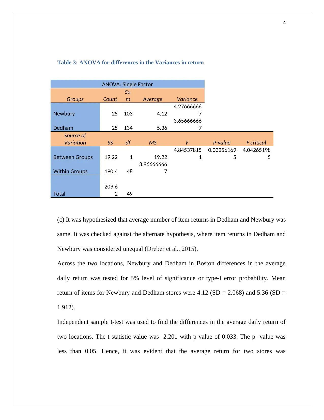
The F-statistic value for the model was 4.845 with p value of 0.033. The p-value was less
than the type-I probability of 0.05. Hence the result of the test was significant. It was
concluded that variances of returns for the two locations was significantly different.

4
Table 3: ANOVA for differences in the Variances in return
ANOVA: Single Factor
Groups Count
Su
m Average Variance
Newbury 25 103 4.12
4.27666666
7
Dedham 25 134 5.36
3.65666666
7
Source of
Variation SS df MS F P-value F critical
Between Groups 19.22 1 19.22
4.84537815
1
0.03256169
5
4.04265198
5
Within Groups 190.4 48
3.96666666
7
Total
209.6
2 49
(c) It was hypothesized that average number of item returns in Dedham and Newbury was
same. It was checked against the alternate hypothesis, where item returns in Dedham and
Newbury was considered unequal (Dreber et al., 2015).
Across the two locations, Newbury and Dedham in Boston differences in the average
daily return was tested for 5% level of significance or type-I error probability. Mean
return of items for Newbury and Dedham stores were 4.12 (SD = 2.068) and 5.36 (SD =
1.912).
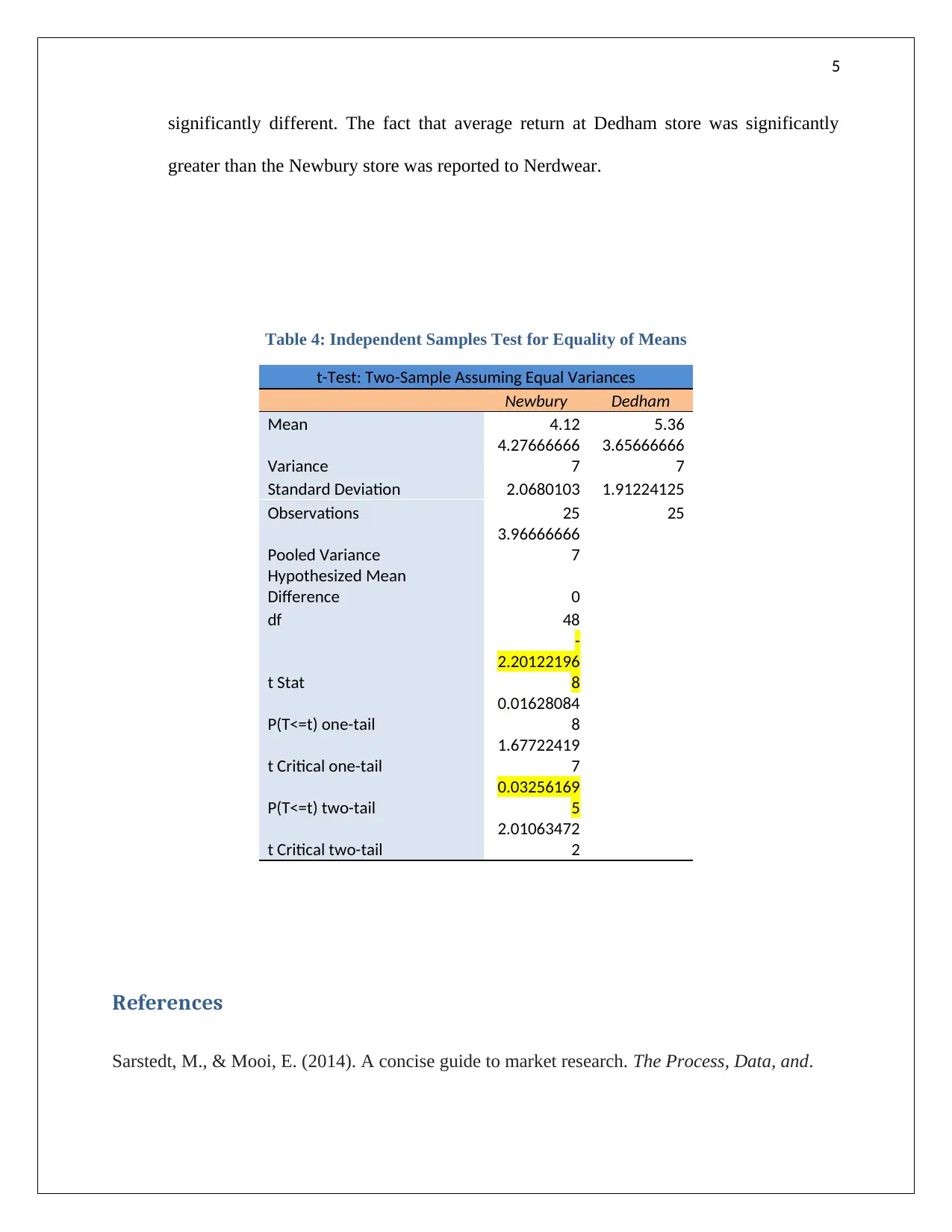
Independent sample t-test was used to find the differences in the average daily return of
two locations. The t-statistic value was -2.201 with p value of 0.033. The p- value was
less than 0.05. Hence, it was evident that the average return for two stores was

5
significantly different. The fact that average return at Dedham store was significantly
greater than the Newbury store was reported to Nerdwear.
Table 4: Independent Samples Test for Equality of Means
t-Test: Two-Sample Assuming Equal Variances
Newbury Dedham
Mean 4.12 5.36
Variance
4.27666666
7
3.65666666
7
Standard Deviation 2.0680103 1.91224125
Observations 25 25
Pooled Variance
3.96666666
7
Hypothesized Mean
Difference 0
df 48
t Stat
-
2.20122196
8
P(T<=t) one-tail
0.01628084
8
t Critical one-tail
1.67722419
7
P(T<=t) two-tail
0.03256169
5
t Critical two-tail
2.01063472
2
References
Sarstedt, M., & Mooi, E. (2014). A concise guide to market research. The Process, Data, and.

6
Dreber, A., Pfeiffer, T., Almenberg, J., Isaksson, S., Wilson, B., Chen, Y., ... & Johannesson, M.
(2015). Using prediction markets to estimate the reproducibility of scientific
research. Proceedings of the National Academy of Sciences, 112(50), 15343-15347.