Statistics Problems and Solutions

The article provides solutions to various statistics problems related to probability, confidence intervals, binomial distribution, Poisson distribution, odds ratio, and logistic regression. The solutions are explained step-by-step to help students understand the concepts better. The problems cover various scenarios such as clinical trials, cancer studies, smoking cessation interventions, and low birthweight investigations.

Surname 1
Student’s Name
Professor’s Name
Course
Date
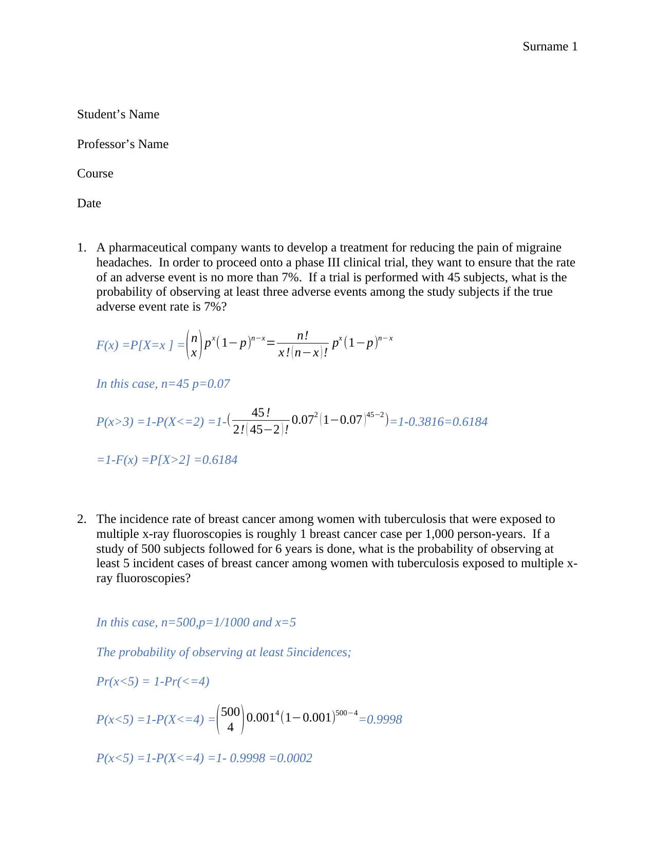
1. A pharmaceutical company wants to develop a treatment for reducing the pain of migraine
headaches. In order to proceed onto a phase III clinical trial, they want to ensure that the rate
of an adverse event is no more than 7%. If a trial is performed with 45 subjects, what is the
probability of observing at least three adverse events among the study subjects if the true
adverse event rate is 7%?
F(x) =P[X=x ] =(n
x ) px( 1− p)n−x= n!
x ! ( n−x ) ! px (1−p)n− x
In this case, n=45 p=0.07
P(x>3) =1-P(X<=2) =1- ( 45 !
2! ( 45−2 ) ! 0.072 ( 1−0.07 ) 45−2 )=1-0.3816=0.6184
=1-F(x) =P[X>2] =0.6184
2. The incidence rate of breast cancer among women with tuberculosis that were exposed to
multiple x-ray fluoroscopies is roughly 1 breast cancer case per 1,000 person-years. If a
study of 500 subjects followed for 6 years is done, what is the probability of observing at
least 5 incident cases of breast cancer among women with tuberculosis exposed to multiple x-
ray fluoroscopies?
In this case, n=500,p=1/1000 and x=5
The probability of observing at least 5incidences;
Pr(x<5) = 1-Pr(<=4)
P(x<5) =1-P(X<=4) = ( 500
4 ) 0.0014 (1−0.001)500−4
=0.9998
P(x<5) =1-P(X<=4) =1- 0.9998 =0.0002

Surname 2
3. Find the 95% confidence interval for the likelihood of a rodent given treatment recovering
from a stroke when thirteen of twenty-one rodents recovered during a recent study.
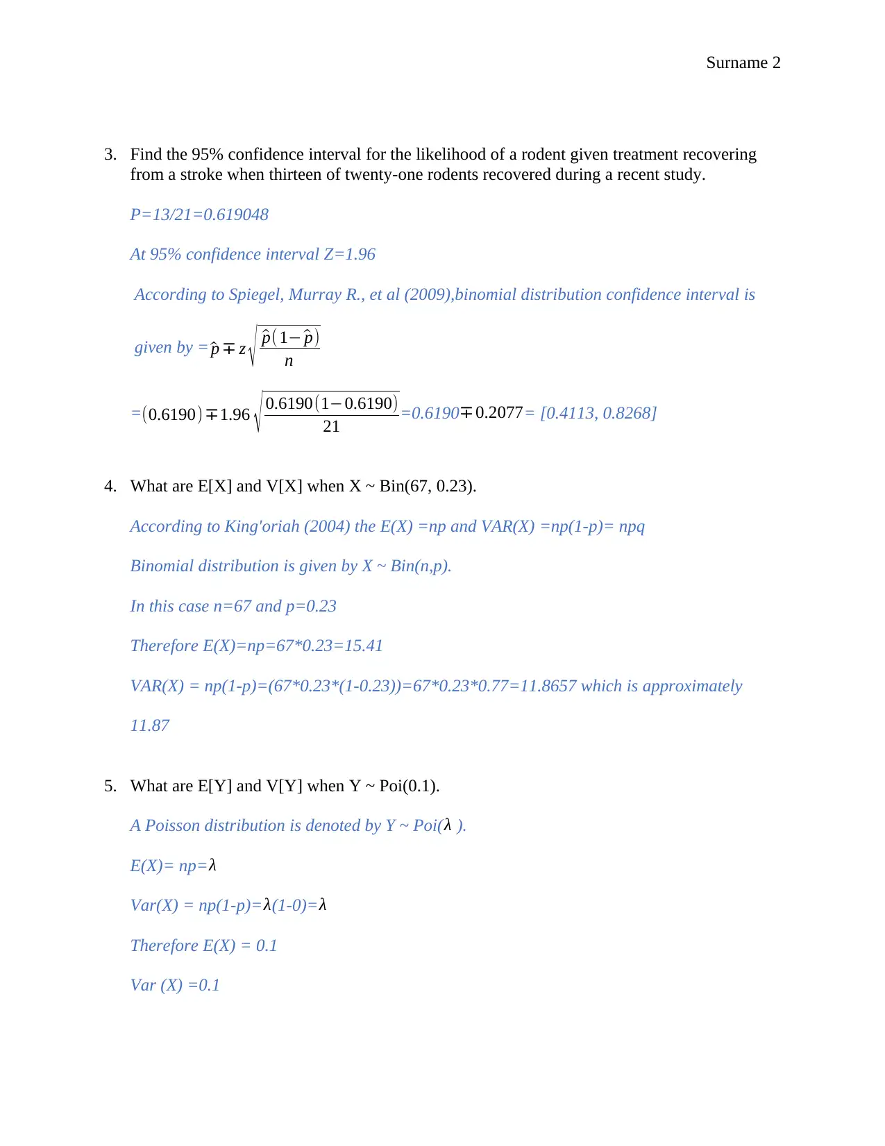
P=13/21=0.619048
At 95% confidence interval Z=1.96
According to Spiegel, Murray R., et al (2009),binomial distribution confidence interval is
given by = ^p ∓ z √ ^p( 1− ^p)
n
=(0.6190) ∓1.96 √ 0.6190(1−0.6190)
21 =0.6190∓ 0.2077= [0.4113, 0.8268]
4. What are E[X] and V[X] when X ~ Bin(67, 0.23).
According to King'oriah (2004) the E(X) =np and VAR(X) =np(1-p)= npq
Binomial distribution is given by X ~ Bin(n,p).
In this case n=67 and p=0.23
Therefore E(X)=np=67*0.23=15.41
VAR(X) = np(1-p)=(67*0.23*(1-0.23))=67*0.23*0.77=11.8657 which is approximately
11.87
5. What are E[Y] and V[Y] when Y ~ Poi(0.1).
A Poisson distribution is denoted by Y ~ Poi(λ ).
E(X)= np=λ
Var(X) = np(1-p)=λ(1-0)=λ
Therefore E(X) = 0.1
Var (X) =0.1

Surname 3
6. The following table describes the relationship between a smoking cessation intervention and
confirmed cessation from smoking. Calculate the odds ratio (90% confidence interval) that
describes the relationship between the intervention and cessation. Interpret your results.
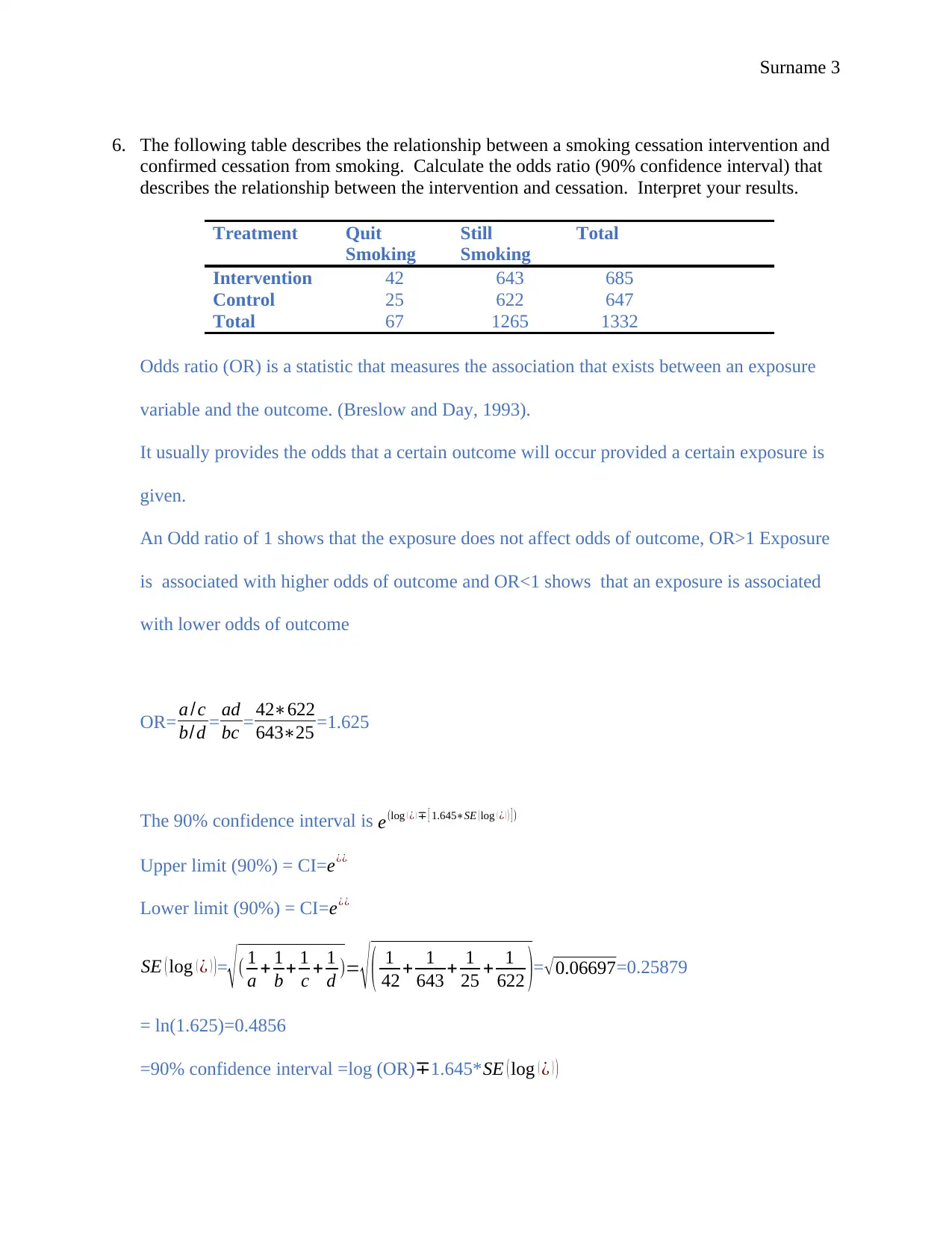
Treatment Quit
Smoking
Still
Smoking
Total
Intervention 42 643 685
Control 25 622 647
Total 67 1265 1332
Odds ratio (OR) is a statistic that measures the association that exists between an exposure
variable and the outcome. (Breslow and Day, 1993).
It usually provides the odds that a certain outcome will occur provided a certain exposure is
given.
An Odd ratio of 1 shows that the exposure does not affect odds of outcome, OR>1 Exposure
is associated with higher odds of outcome and OR<1 shows that an exposure is associated
with lower odds of outcome
OR= a /c
b/ d = ad
bc = 42∗622
643∗25 =1.625
The 90% confidence interval is e(log ( ¿ ) ∓ [ 1.645∗SE ( log ( ¿ ) ) ] )
Upper limit (90%) = CI=e¿¿
Lower limit (90%) = CI= e¿¿
SE ( log ( ¿ ) )=
√( 1
a + 1
b + 1
c + 1
d )= √ ( 1
42 + 1
643 + 1
25 + 1
622 )=√0.06697=0.25879
= ln(1.625)=0.4856
=90% confidence interval =log (OR)∓1.645*SE ( log ( ¿ ) )

Surname 4
=log 90% confidence interval =0.4856 ∓1.645*0.25879= (0.05988, 0.9113)
Lower limit =Exp (0.05988) =1.062
Upper limit= Exp (0.9113) =2.488
ANS [1.062,2.488]
7. Find the relative risk and 90% confidence interval for the table used above (in problem 6).
Interpret these results, and compare them to the results of problem 6.
According to the finding of Altman (1991) the relative risk is given by
RR= a/( a+b)
c /( c+ d)= 42/(42+643)
25/(25+622) =1.5868
= The 90% confidence interval is e(ln ( RR ) ∓ [ 1.645∗SE ( ln ( RR ) ) ] )
Where SE ( ln ( RR ) )=
√( 1
a + 1
c − 1
a+b − 1
c +d )
Deeks & Higgins (2010);Pagano & Gauvreau (2000) advises that in situation where zeros
may cause problem in computation of relative risk a value of 0.5 is added to a, b, c and d
cells.
SE ( ln ( RR ) )=
√ ( 1
42 + 1
25 − 1
42+643 − 1
25+622 )=√0.060804= 0.2466
=ln(RR)=ln(1.5868)=0.4617
log 90% confidence interval =0.4617 ∓1.645*0.466 = (0.05609, 0.8674)
Lower limit =Exp (0.05609) =1.058
Upper limit= Exp (0.8674) =2.381
ANS [1.058, 2.381]

Surname 5
8. Investigators are study poisoning among children by two different drugs that were the
leading cause of death in child poisoning cases, drug A and drug B. Of interest was whether
or not the child was responsible for the accident. The summary table is given below.
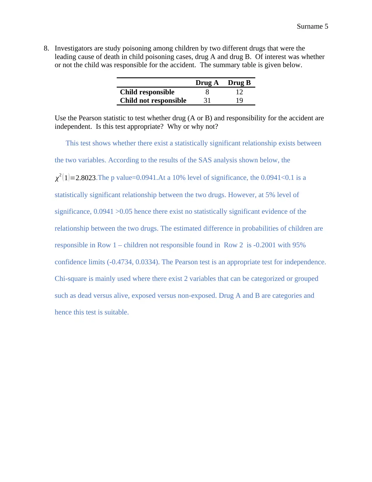
Drug A Drug B
Child responsible 8 12
Child not responsible 31 19
Use the Pearson statistic to test whether drug (A or B) and responsibility for the accident are
independent. Is this test appropriate? Why or why not?
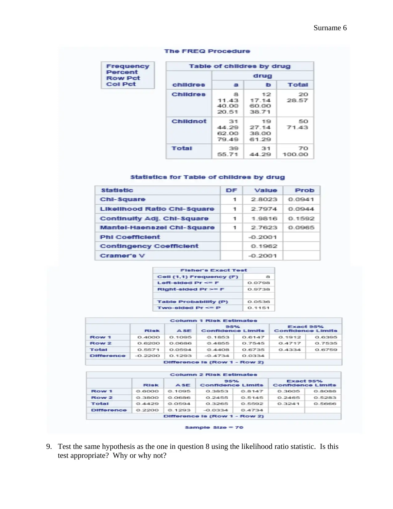
This test shows whether there exist a statistically significant relationship exists between
the two variables. According to the results of the SAS analysis shown below, the
χ2 ( 1 ) =2.8023.The p value=0.0941.At a 10% level of significance, the 0.0941<0.1 is a
statistically significant relationship between the two drugs. However, at 5% level of
significance, 0.0941 >0.05 hence there exist no statistically significant evidence of the
relationship between the two drugs. The estimated difference in probabilities of children are
responsible in Row 1 – children not responsible found in Row 2 is -0.2001 with 95%
confidence limits (-0.4734, 0.0334). The Pearson test is an appropriate test for independence.
Chi-square is mainly used where there exist 2 variables that can be categorized or grouped
such as dead versus alive, exposed versus non-exposed. Drug A and B are categories and
hence this test is suitable.

Surname 6
9. Test the same hypothesis as the one in question 8 using the likelihood ratio statistic. Is this
test appropriate? Why or why not?

Surname 7
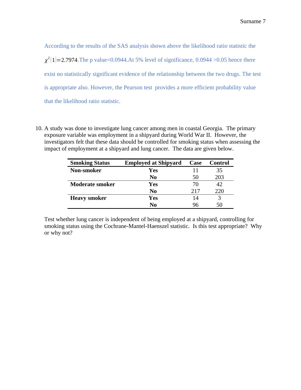
According to the results of the SAS analysis shown above the likelihood ratio statistic the
χ2 ( 1 )=2.7974.The p value=0.0944.At 5% level of significance, 0.0944 >0.05 hence there
exist no statistically significant evidence of the relationship between the two drugs. The test
is appropriate also. However, the Pearson test provides a more efficient probability value
that the likelihood ratio statistic.
10. A study was done to investigate lung cancer among men in coastal Georgia. The primary
exposure variable was employment in a shipyard during World War II. However, the
investigators felt that these data should be controlled for smoking status when assessing the
impact of employment at a shipyard and lung cancer. The data are given below.
Smoking Status Employed at Shipyard Case Control
Non-smoker Yes 11 35
No 50 203
Moderate smoker Yes 70 42
No 217 220
Heavy smoker Yes 14 3
No 96 50
Test whether lung cancer is independent of being employed at a shipyard, controlling for
smoking status using the Cochrane-Mantel-Haenszel statistic. Is this test appropriate? Why
or why not?

Surname 8
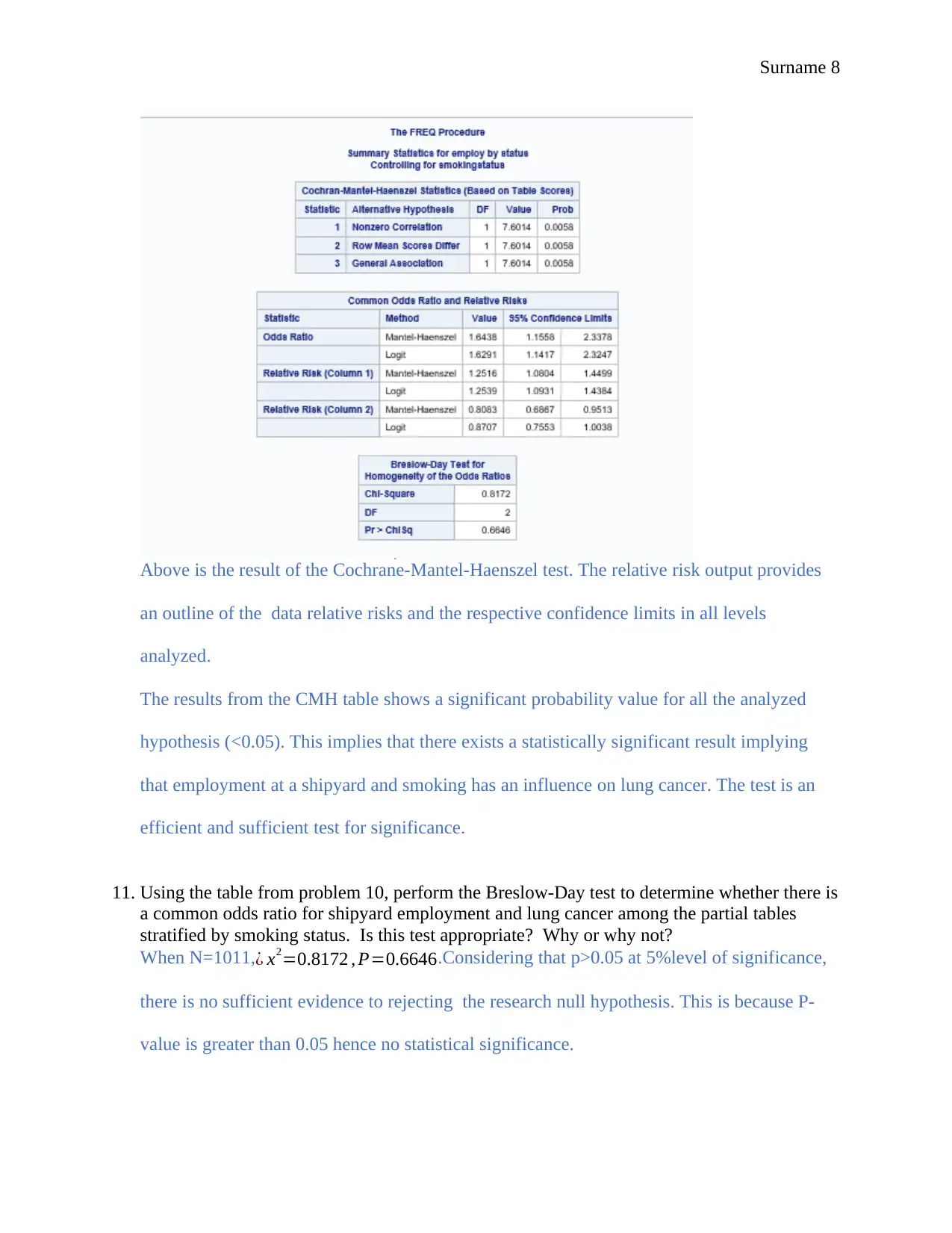
Above is the result of the Cochrane-Mantel-Haenszel test. The relative risk output provides
an outline of the data relative risks and the respective confidence limits in all levels
analyzed.
The results from the CMH table shows a significant probability value for all the analyzed
hypothesis (<0.05). This implies that there exists a statistically significant result implying
that employment at a shipyard and smoking has an influence on lung cancer. The test is an
efficient and sufficient test for significance.
11. Using the table from problem 10, perform the Breslow-Day test to determine whether there is
a common odds ratio for shipyard employment and lung cancer among the partial tables
stratified by smoking status. Is this test appropriate? Why or why not?
When N=1011,¿ x2=0.8172 , P=0.6646.Considering that p>0.05 at 5%level of significance,
there is no sufficient evidence to rejecting the research null hypothesis. This is because P-
value is greater than 0.05 hence no statistical significance.

Surname 9
Considering this, there is no enough evidence of an effect of modification, therefore the
smoking status relative odd is similar. There is, therefore, a common odds ratio for shipyard
employment and lung cancer among the partial tables stratified by smoking status
12. Using the table from problem 10, assume that the true odds ratio of shipyard employment and
lung cancer is the same across the partial tables that stratified by smoking status. Find an
estimate of the common odds ratio along with its corresponding 95% confidence interval.
According to the figure above the relative risk of lung cancer is 1.2539 that has a 95%
confidence interval (CI=1.0931, 1.4384). The odds ratio is found in the first column in the
common odds ratio and relative risk table. OR=1.6291.The confidence intervals were CI=
(1.1417, 2.3247).
13. Using the table from problem 10, run a logistic regression model that fits the conditional
odds model. Do shipyard employment and smoking status need to be included in this model?
Why or why not? Does this model fit the data?
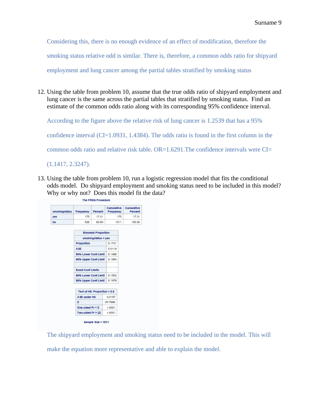
The shipyard employment and smoking status need to be included in the model. This will
make the equation more representative and able to explain the model.

Surname 10
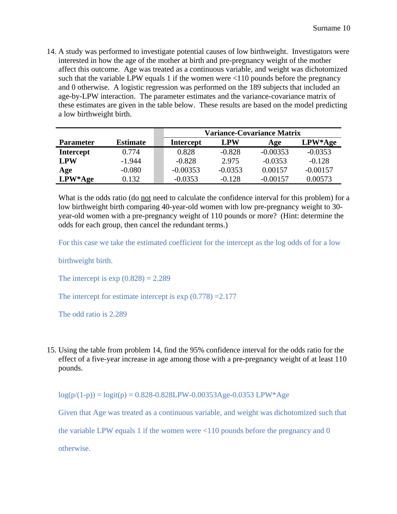
14. A study was performed to investigate potential causes of low birthweight. Investigators were
interested in how the age of the mother at birth and pre-pregnancy weight of the mother
affect this outcome. Age was treated as a continuous variable, and weight was dichotomized
such that the variable LPW equals 1 if the women were <110 pounds before the pregnancy
and 0 otherwise. A logistic regression was performed on the 189 subjects that included an
age-by-LPW interaction. The parameter estimates and the variance-covariance matrix of
these estimates are given in the table below. These results are based on the model predicting
a low birthweight birth.
Variance-Covariance Matrix
Parameter Estimate Intercept LPW Age LPW*Age
Intercept 0.774 0.828 -0.828 -0.00353 -0.0353
LPW -1.944 -0.828 2.975 -0.0353 -0.128
Age -0.080 -0.00353 -0.0353 0.00157 -0.00157
LPW*Age 0.132 -0.0353 -0.128 -0.00157 0.00573
What is the odds ratio (do not need to calculate the confidence interval for this problem) for a
low birthweight birth comparing 40-year-old women with low pre-pregnancy weight to 30-
year-old women with a pre-pregnancy weight of 110 pounds or more? (Hint: determine the
odds for each group, then cancel the redundant terms.)
For this case we take the estimated coefficient for the intercept as the log odds of for a low
birthweight birth.
The intercept is exp (0.828) = 2.289
The intercept for estimate intercept is exp (0.778) =2.177
The odd ratio is 2.289
15. Using the table from problem 14, find the 95% confidence interval for the odds ratio for the
effect of a five-year increase in age among those with a pre-pregnancy weight of at least 110
pounds.
log(p/(1-p)) = logit(p) = 0.828-0.828LPW-0.00353Age-0.0353 LPW*Age
Given that Age was treated as a continuous variable, and weight was dichotomized such that
the variable LPW equals 1 if the women were <110 pounds before the pregnancy and 0
otherwise.

Surname 11
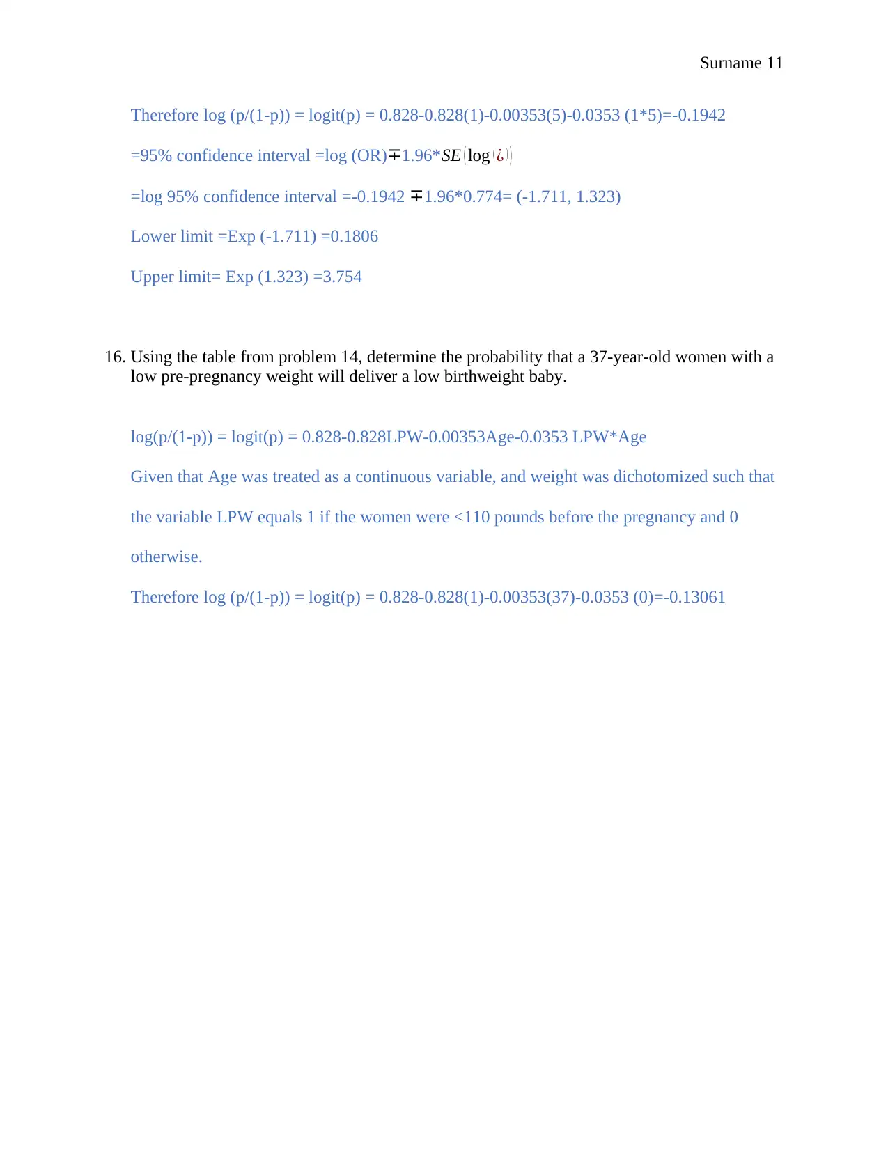
Therefore log (p/(1-p)) = logit(p) = 0.828-0.828(1)-0.00353(5)-0.0353 (1*5)=-0.1942
=95% confidence interval =log (OR)∓1.96*SE ( log ( ¿ ) )
=log 95% confidence interval =-0.1942 ∓1.96*0.774= (-1.711, 1.323)
Lower limit =Exp (-1.711) =0.1806
Upper limit= Exp (1.323) =3.754
16. Using the table from problem 14, determine the probability that a 37-year-old women with a
low pre-pregnancy weight will deliver a low birthweight baby.
log(p/(1-p)) = logit(p) = 0.828-0.828LPW-0.00353Age-0.0353 LPW*Age
Given that Age was treated as a continuous variable, and weight was dichotomized such that
the variable LPW equals 1 if the women were <110 pounds before the pregnancy and 0
otherwise.
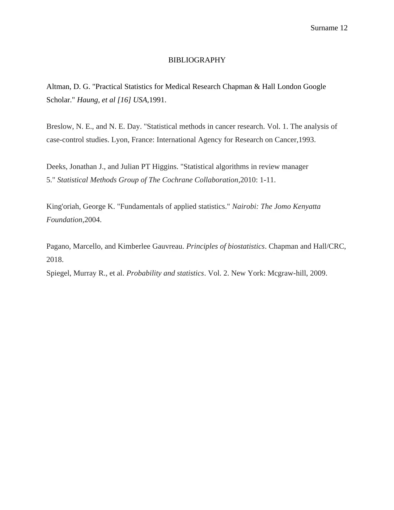
Therefore log (p/(1-p)) = logit(p) = 0.828-0.828(1)-0.00353(37)-0.0353 (0)=-0.13061

Surname 12
BIBLIOGRAPHY
Altman, D. G. "Practical Statistics for Medical Research Chapman & Hall London Google
Scholar." Haung, et al [16] USA,1991.
Breslow, N. E., and N. E. Day. "Statistical methods in cancer research. Vol. 1. The analysis of
case-control studies. Lyon, France: International Agency for Research on Cancer,1993.
Deeks, Jonathan J., and Julian PT Higgins. "Statistical algorithms in review manager
5." Statistical Methods Group of The Cochrane Collaboration,2010: 1-11.
King'oriah, George K. "Fundamentals of applied statistics." Nairobi: The Jomo Kenyatta
Foundation,2004.
Pagano, Marcello, and Kimberlee Gauvreau. Principles of biostatistics. Chapman and Hall/CRC,
2018.
Spiegel, Murray R., et al. Probability and statistics. Vol. 2. New York: Mcgraw-hill, 2009.