Statistics Assignment: Analysis of Australian Exports, Frequency Table, Time Series, Correlation Analysis and Linear Regression

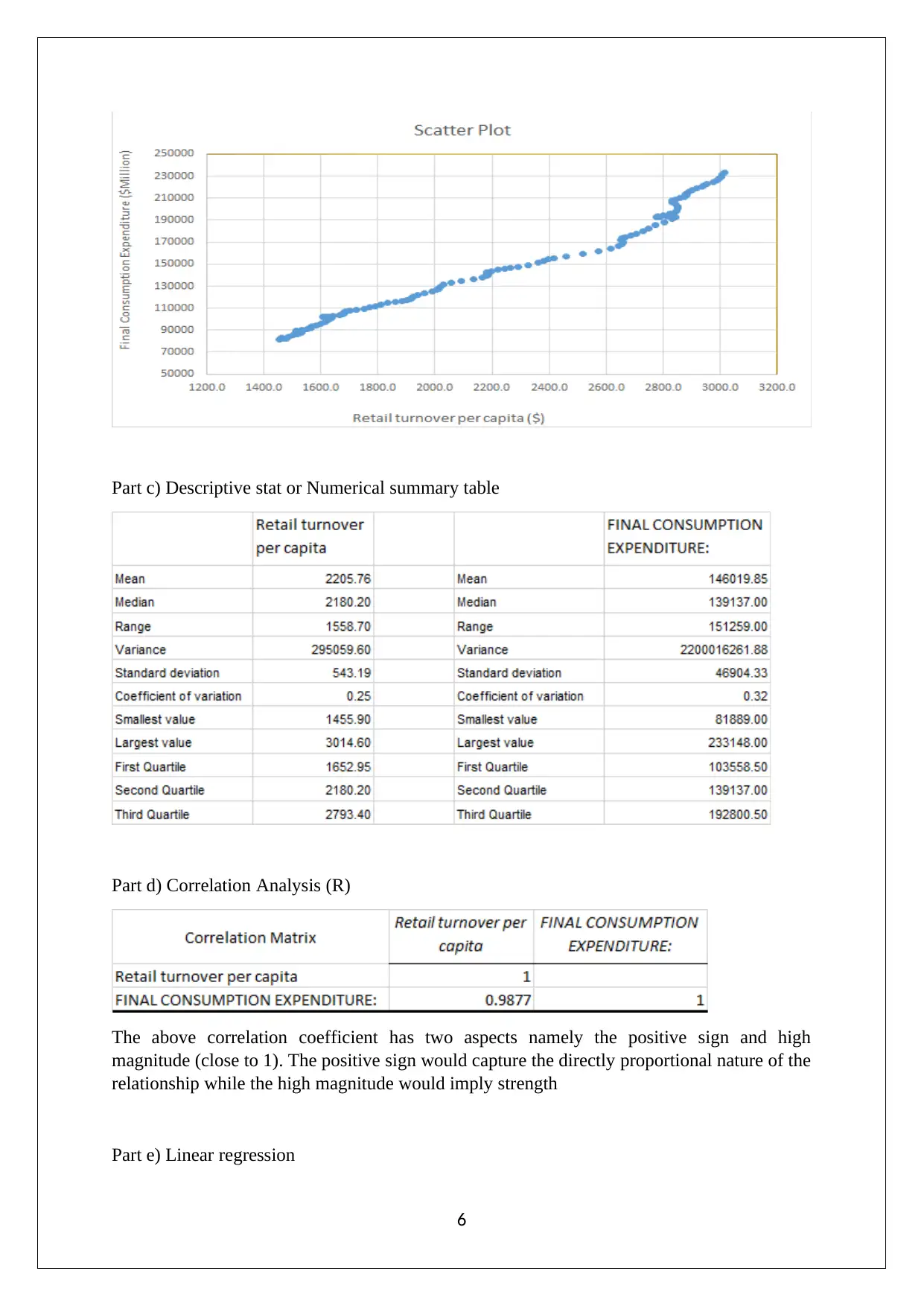
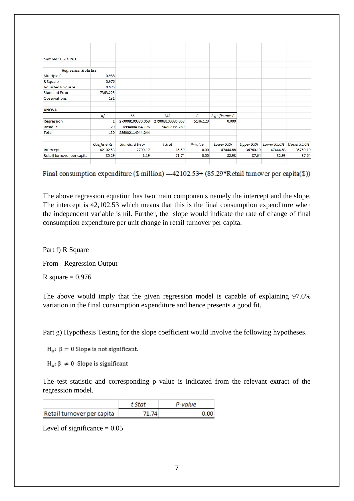
This Statistics assignment covers the analysis of Australian exports, frequency table, time series, correlation analysis, and linear regression. The assignment includes graphical illustrations, frequency tables, relative frequency histogram, Ogive, numerical summary table, correlation analysis, linear regression, and hypothesis testing. The assignment also covers the interpretation of the results obtained from the analysis.

STATISTICS
STUDENT ID:
[Pick the date]

Question 1
Part a) Direction of exports values for Australia is represented below.
Part b) Australian – Direction of exports (%)
For 2004/2005 For 2014/2015
Part c) Taking into reference the above graphical illustrations, following aspects would be
highlighted.
 China has grown its share in Australian exports at a rapid pace which is apparent from
the significant jump in share during the 10 year period. As a result, the share of every
other country in the Australian exports has seen a fall in their share even though some
of them have witnessed higher absolute exports from Australia.
 There is a noticeable exception to the rising exports from Australia to each of the
trade partners considered above. This exception is in the form of United Kingdom
since it has been a fall in exports from Australia during the 10 year period which is
surprising.
2

 Another key observation relates to the stagnant exports from Australia headed to New
Zealand. It is interesting to see exports from Australia increased to far off trade
partners such as India and China but it has not increased with New Zealand despite
the minimal distance and logistics cost involved.
Question 2
Part a) Frequency table (Umbrella Sold)
Classes Frequency Relative Frequency
30-40 2 0.05
40-50 4 0.10
50-60 8 0.20
60-70 11 0.28
70-80 8 0.20
80-90 5 0.13
90-100 2 0.05
Part b) Frequency table (Umbrella Sold)
Part c) Relative Frequency Histogram
3

Part d) Ogive
Part e) Proportion of umbrella sold < than 60
= (2/40) + (4/40) + (8/40) = 0.35
4

Part f) Proportion of umbrella sold >more than 70
= (8/40) +(5/40) + (2/40) = 0.38
Question 3
Part a) Time series through line chart
Part b) Scatter display for relationship between the given variables has been drawn using
Excel. The dependent variable is the final consumption expenditure which is represented on
the Y axis. The independent variable is the retail turnover per person which finds
representation on theX axis.
5

Part c) Descriptive stat or Numerical summary table
Part d) Correlation Analysis (R)
The above correlation coefficient has two aspects namely the positive sign and high
magnitude (close to 1). The positive sign would capture the directly proportional nature of the
relationship while the high magnitude would imply strength
Part e) Linear regression
6

The above regression equation has two main components namely the intercept and the slope.
The intercept is 42,102.53 which means that this is the final consumption expenditure when
the independent variable is nil. Further, the slope would indicate the rate of change of final
consumption expenditure per unit change in retail turnover per capita.
Part f) R Square
From - Regression Output
R square = 0.976
The above would imply that the given regression model is capable of explaining 97.6%
variation in the final consumption expenditure and hence presents a good fit.
Part g) Hypothesis Testing for the slope coefficient would involve the following hypotheses.
The test statistic and corresponding p value is indicated from the relevant extract of the
regression model.
Level of significance = 0.05
7

Comparing the p value and significance level, it is apparent that the greater value if level of
significance, which would lead to H0 rejection and H1 acceptance. As a result, the
significance of the slope coefficient is established.
Part h) Standard error
From - Regression Output
Standard error = 7363.225
The standard error is indicative of the level of fit of the model as a good fit would have low
standard error. This is because deviation between expected values and actual values would be
minimal. This is the case here and thereby it would be fair to conclude the regression model
as a reasonable fit.
8