Statistics: Simple Linear Regression and Multiple Regression Analysis

This document provides an overview of simple linear regression and multiple regression analysis in statistics. It explains the statistical models, assumptions, and interpretation of the regression models. The document also covers topics such as predicting and validating regression models. It is a useful resource for students studying statistics.

Statistics
Student Name:
Date: 23rd May 2019

Question 1 [28 marks]
a. [3 marks] State the statistical model for a simple linear regression of Extent explained by
Year. Carefully define all the necessary variables and parameters in your answer.
Answer
The statistical model for a simple linear regression is given as follows;
Extent=β0 + β1 ( Year ) +ε
Where β0=constant (Intercept )coefficient
β1=coefficient of the year
ε =error term
Extent is the response (dependent) variable while year is the explanatory (independent)
variable
b. [3 marks] A simple linear regression seems appropriate for the 1979-2002 data. Justify
the use of a simple linear regression model.
Answer
A simple linear regression is appropriate because we only have one explanatory variable
which is the year otherwise if we had more than one explanatory variable then multiple
regression would have been appropriate.
c. [2 marks] Fit a simple linear regression to the 1979-2002 data. Explain why there is a
linear relationship.
Answer
> regmodel= lm(Extent
~ Year, data = data)
> summary(regmodel)
Call:
lm(formula = Extent ~
Year, data = data)
Residuals:
Min 1Q Median
3Q Max
-1.31813 -0.38533
0.03363 0.39009
1.29284
Coefficients:
Estimate Std.
Error t value Pr(>|t|)
(Intercept) 180.815939
19.796988 9.134 1.98e-
10 ***
Year -0.087439
0.009921 -8.814 4.53e-
10 ***
---

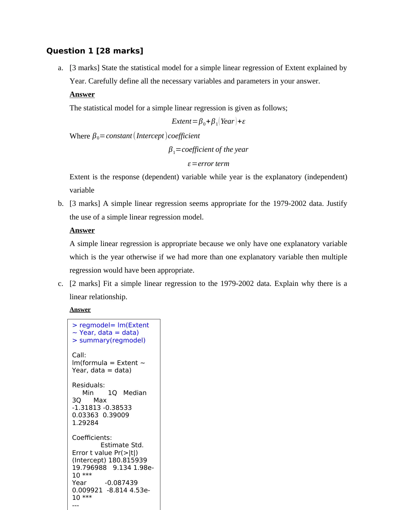
We have the regression model as;
Extent=180.8159−0.0874 ( Year )
No there is no linear relationship based on the scatter plot above. The plot shows that
there is no linear relationship between the two variables.
d. [2 marks] Is this a strong linear relationship? Explain your answer in the context of this
data.
Answer
Yes this is a strong negative linear relationship. This is based on the value of R is -0.8416
which shows a strong negative relationship between the variables.
e. [2 marks] Predict the extent of the sea ice (in km2) for the year 2000.
Answer
Given the year as 2000 we can predict the extent as follows;
Extent=180.8159−0.0874 ( 2000 )
Extent=180.8159−174.8=6.0159
Thus the predicted Extent for the year 2000 is 6.0159.
f. [2 marks] Compute a 95% prediction band for the Extent of Sea Ice (in km2) in the year
2000.
Answer

g. [2 marks] Compute a 95% confidence band for the Extent
of Sea Ice (in km2) in the year 2000.
Answer
h. [2 marks] Explain clearly what the prediction band
represents and what the confidence band represents.
Answer
The 95% prediction band is between 4.761 and 7.114 while we are 95% confident that
the confidence band is between 5.719 and 6.156.
i. [2 marks] Justify why a simple linear regression is inappropriate for the 1979-2012 data.
Answer
Simple linear regression is not appropriate since the data is not linear. Simple regression
is not appropriate for a non-linear data
j. [3 marks] Fit a second order polynomial regression model to the data and validate the
model.
Answer
> newdata =
data.frame(Year=2000)
> predict(regmodel,
newdata,
interval="predict")
fit lwr upr
1 5.937406 4.761006
7.113805
> newdata =
data.frame(Year=2000)
> predict(regmodel,
newdata,
interval="confidence")
fit lwr upr
1 5.937406 5.719292
6.155519
> polmodel <- lm(Extent
~ poly(Year,2))
> summary(polmodel)
Call:
lm(formula = Extent ~
poly(Year, 2))
Residuals:
Min 1Q Median
3Q Max
-0.9300 -0.2932 0.0938
0.2796 0.9173
Coefficients:
Estimate Std.
Error t value Pr(>|t|)
(Intercept) 6.33088
0.07829 80.869 < 2e-16
***
poly(Year, 2)1 -5.00203
0.45648 -10.958 3.45e-
12 ***
poly(Year, 2)2 -1.96136
0.45648 -4.297
0.000159 ***

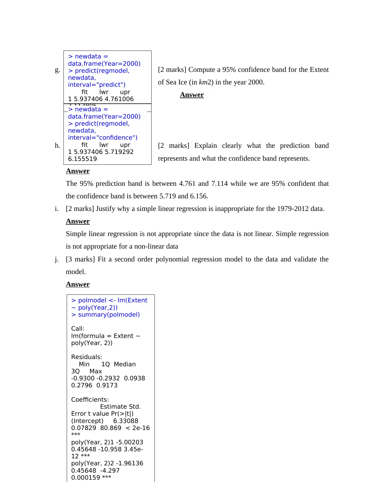
k. [1 mark] Plot the fitted polynomial to your data
Answer
l. [2 marks] Using the second order model you fitted, predict the extent of the sea ice (in
km2) for the year 2000.
Answer
Given the year as 2000 we can predict the extent as follows;
Extent=6.33088−5.00203 ( Year ) −1.96136 ( Year ) 2
Extent=6.33088−5.00203 ( 2000 ) −1.96136 ( 2000 ) 2
Extent=7.056
Thus the predicted Extent for the year 2000 is 7.056.
m. [2 marks] Compare your answers in part e) and part l). Which prediction value do you
recommend and why?
Answer
The prediction value using the polynomial of second order is the most appropriate as
compared to that of the simple regression. This is because the prediction with the
polynomial is closer to the actual than that of the simple regression.

Question 2 [25 marks]
a. [4 marks] State the statistical model for a multiple regression with Quality as the response
using all other variables as predictors, defining any parameters as necessary.
Answer
The statistical model for a simple linear regression is given as follows;
Quality=β0 + β1 ( Alcohol ) + β2 ( Density )+ β3 ( PH )+ ε
Where β0=constant (Intercept )coefficient
β1=coefficient for the Alcohol , β2=coefficient for the density , β3 =coefficient for the PH
ε =error term
Quality is the response (dependent) variable while alcohol, density and PH are the
explanatory (independent) variables
b. [2 marks] Fit this multiple regression model and write down the fitted model.
Answer
The fitted model is given as follows;
> multreg=lm(Quality ~
Alcohol+Density+pH,
data=data1)
> summary(multreg)
Call:
lm(formula = Quality ~
Alcohol + Density + pH,
data = data1)
Residuals:
Min 1Q Median
3Q Max
-3.08673 -0.48594 -
0.02876 0.49009
2.28924
Coefficients:
Estimate Std.
Error t value Pr(>|t|)
(Intercept) -46.18943
31.03540 -1.488
0.13779
Alcohol 0.38190
0.04723 8.086 1.83e-14
***
Density 51.33496
30.50312 1.683
0.09349 .
pH -0.84169
0.31418 -2.679 0.00782
**
---
Signif. codes: 0 ‘***’
0.001 ‘**’ 0.01 ‘*’ 0.05 ‘.’
0.1 ‘ ’ 1

Quality=−46.1894+0.3819 ( Alcohol ) +51.335 ( Density )−0.8417 ( PH )
c. [4 marks] What are the assumptions required for a multiple regression analysis? If
possible, validate those assumptions for the multiple regression model you fitted in part
b.
Answer
The assumptions required for the multiple regressions include;
 Normality of the residual terms
 Linearity
 Homoscedasticity of the residual terms
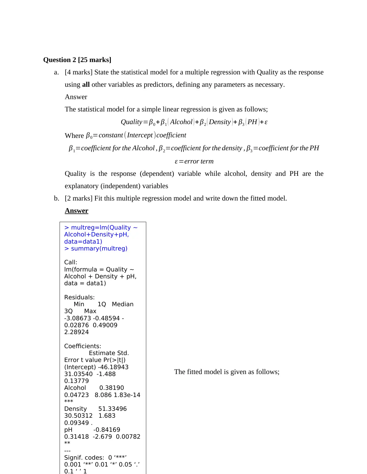
Normality of the residual terms
The figure below shows that the residual terms follow a normal distribution as they are
clustered on a straight line.
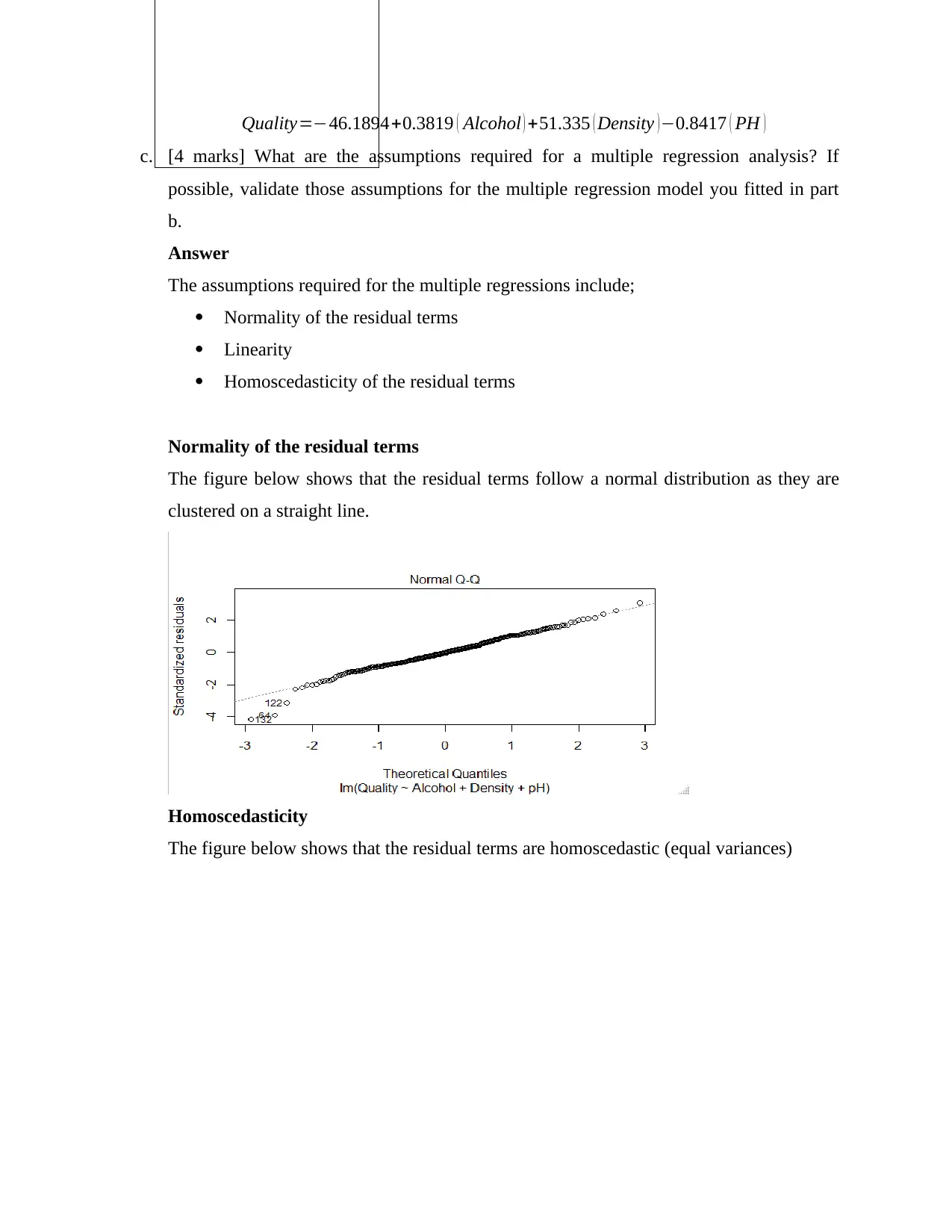
Homoscedasticity
The figure below shows that the residual terms are homoscedastic (equal variances)

d. [6 marks] Conduct an F-test for the overall regression i.e. is there any relationship
between the response and the predictors. Write your answer as a formal hypothesis test
and include the ANOVA table (one combined regression SS source is sufficient.)
Answer
To test for the overall regression i.e. is there any relationship between the response and
the predictors the following hypothesis is tested;
Null hypothesis (H0): There is no relationship between the response and the predictors
Alternative hypothesis (HA): There is relationship between the response and the
predictors.

From the regression analysis, the summary table presented above showed that the overall
model is significant at 5% level of significance [f(3, 282) = 26.22, p = 0.000].
e. [3 marks] From the analysis in part b. determine the 95% CI for the Alcohol slope
parameter and comment on its meaning in this context.
Answer
From the above computation, we are 95%
confident that the alcohol slope is between 0.2610 and 0.4208
f. [2 marks] Using the model selection procedures used in this course, find the best multiple
regression model that explains the data giving reasons for your choice(s).
Answer
The best multiple regression model is that that has Alcohol and pH as the predictor
variables. This is because the Density was found to be insignificant in the model.
g. [4 marks] State the final fitted regression model and comment on its interpretation.
Answer
The final fitted model is given as follows;
> multreg=lm(Quality ~
Alcohol+pH, data=data1)
> summary(multreg)
Call:
lm(formula = Quality ~
Alcohol + pH, data =
data1)
Residuals:
Min 1Q Median
3Q Max
-2.91877 -0.48746 -
0.02972 0.47298
2.26891
Coefficients:
Estimate Std.
Error t value Pr(>|t|)
(Intercept) 6.0141
1.0063 5.977 6.84e-09
***
Alcohol 0.3409
0.0406 8.397 2.23e-15
***
pH -1.0260
0.2954 -3.473 0.000596
***
---
> library(ISwR)
> confint(multreg,
'Alcohol', level=0.95)
2.5 % 97.5 %
Alcohol 0.2610127
0.4208463

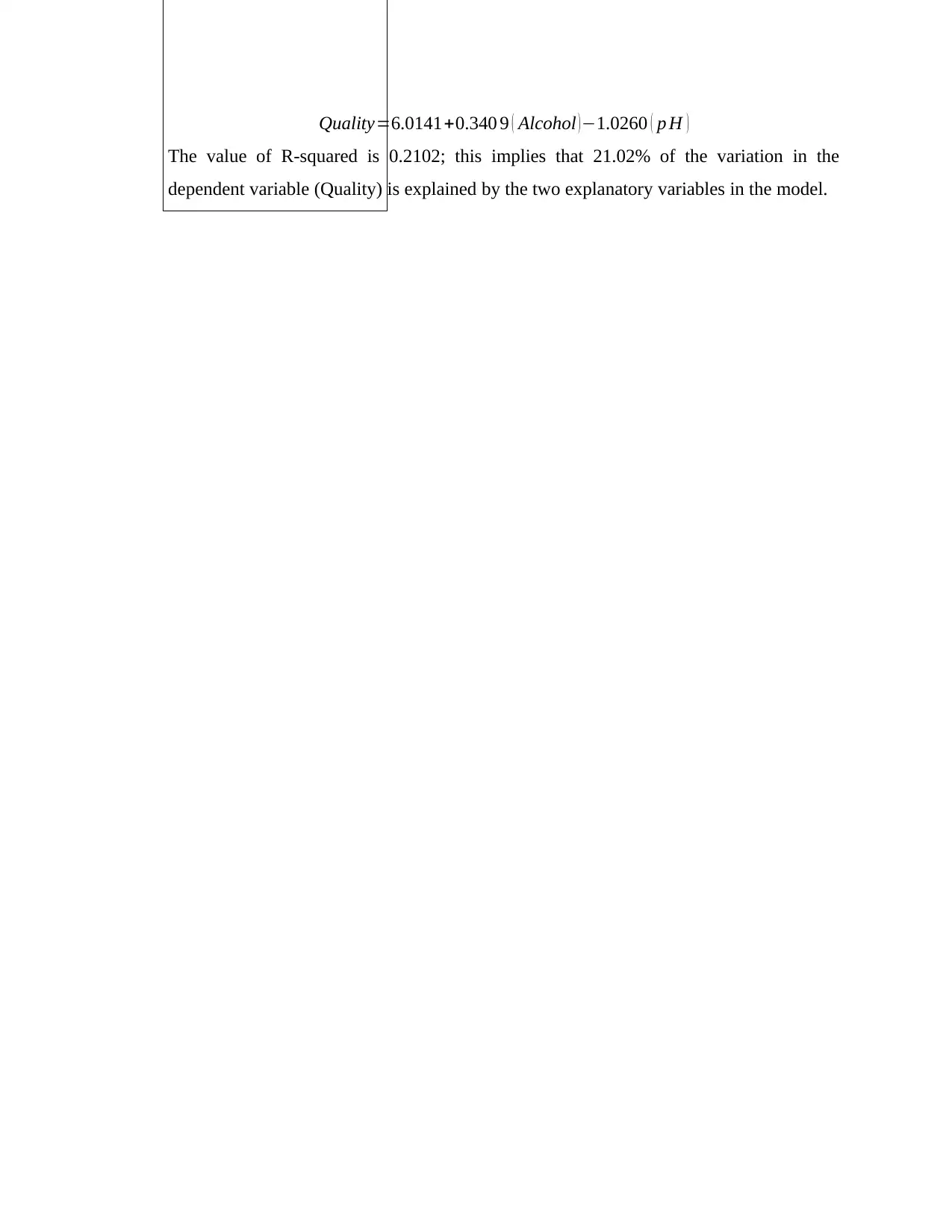
Quality=6.0141+0.340 9 ( Alcohol )−1.0260 ( p H )
The value of R-squared is 0.2102; this implies that 21.02% of the variation in the
dependent variable (Quality) is explained by the two explanatory variables in the model.