Statistical Analysis of Real Estate Market Data Report

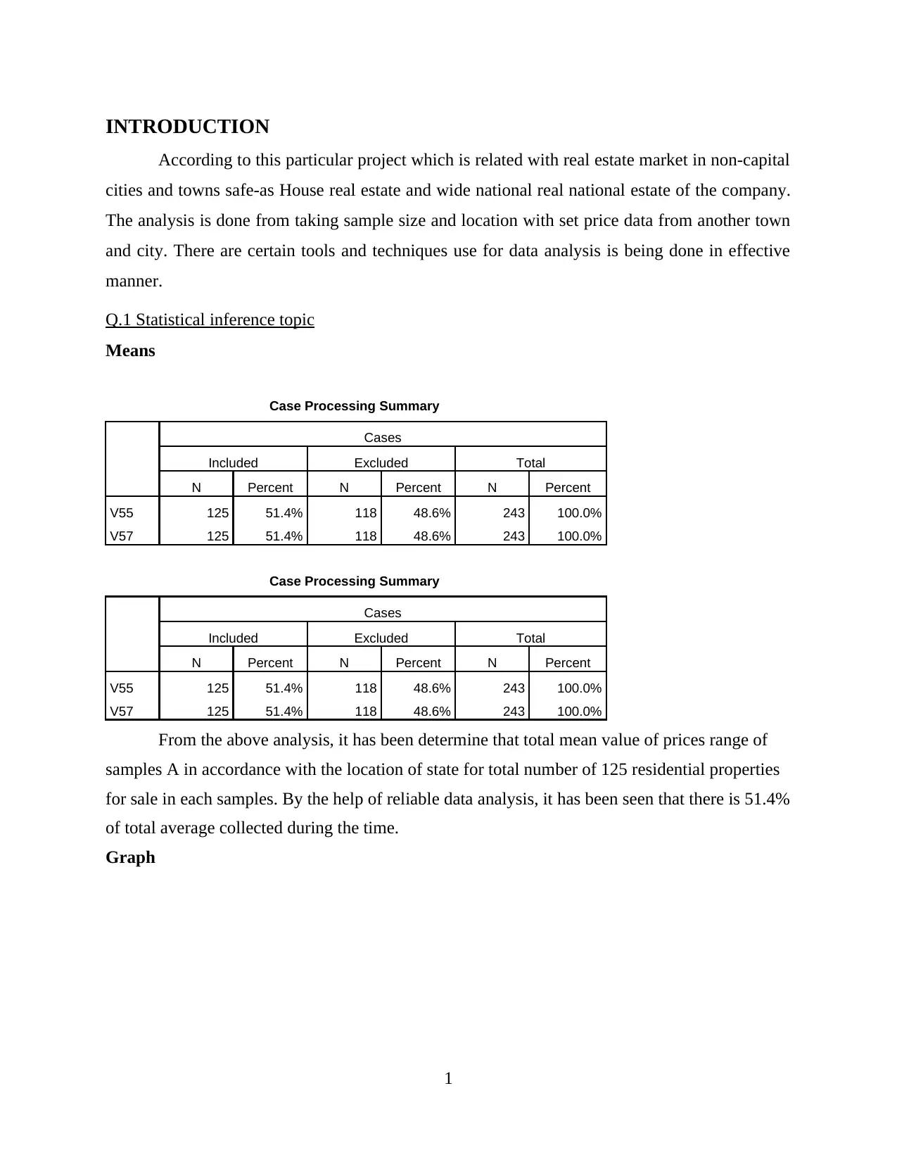
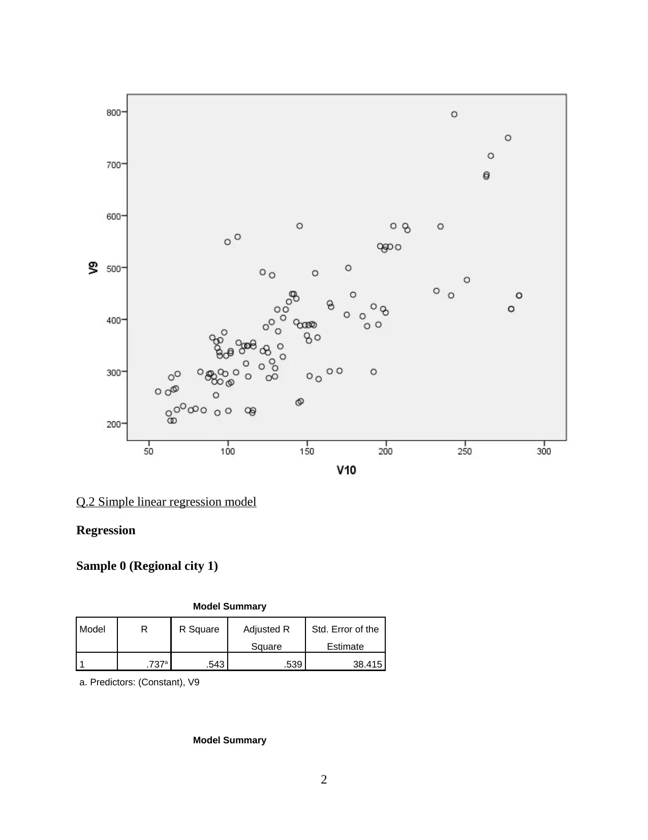
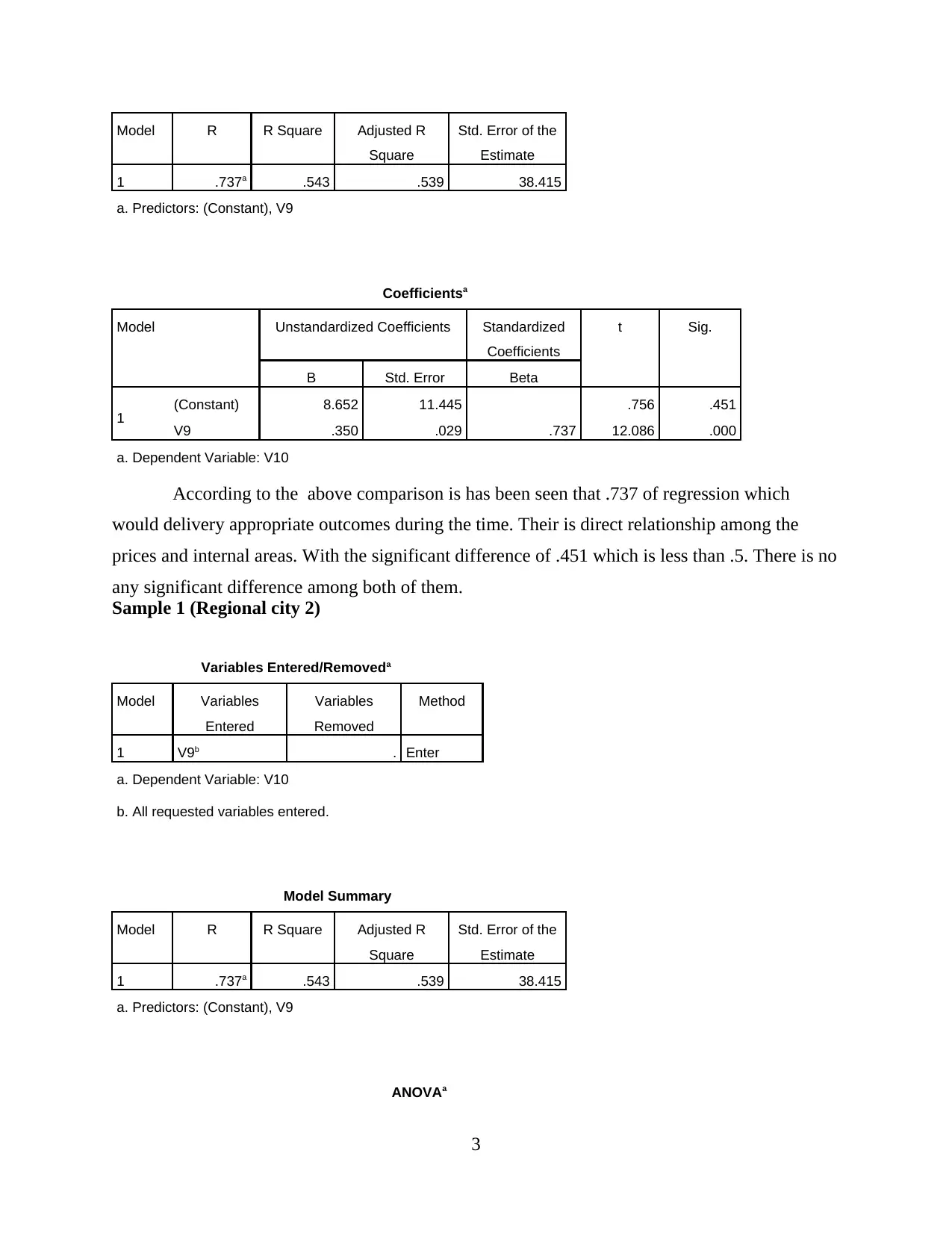
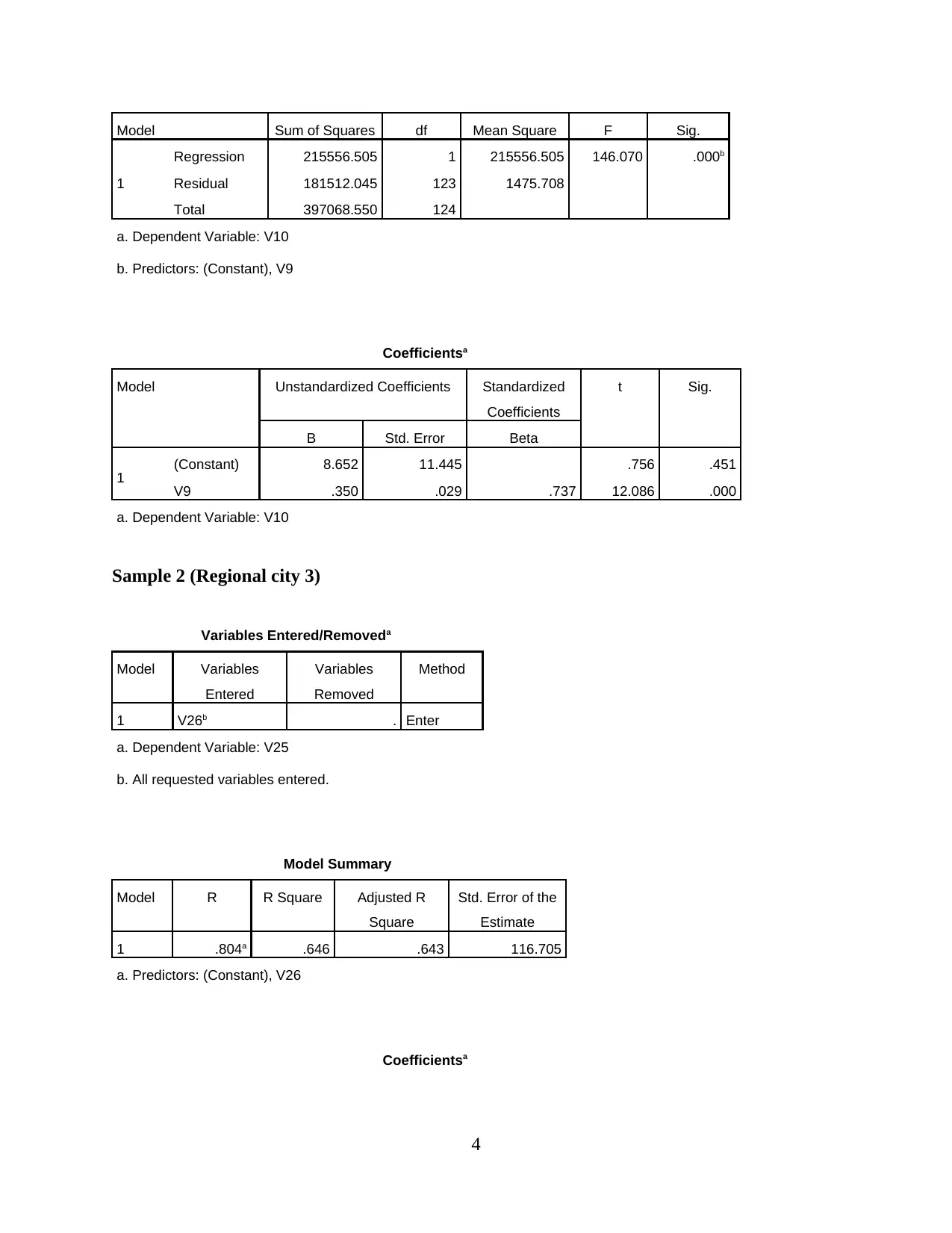
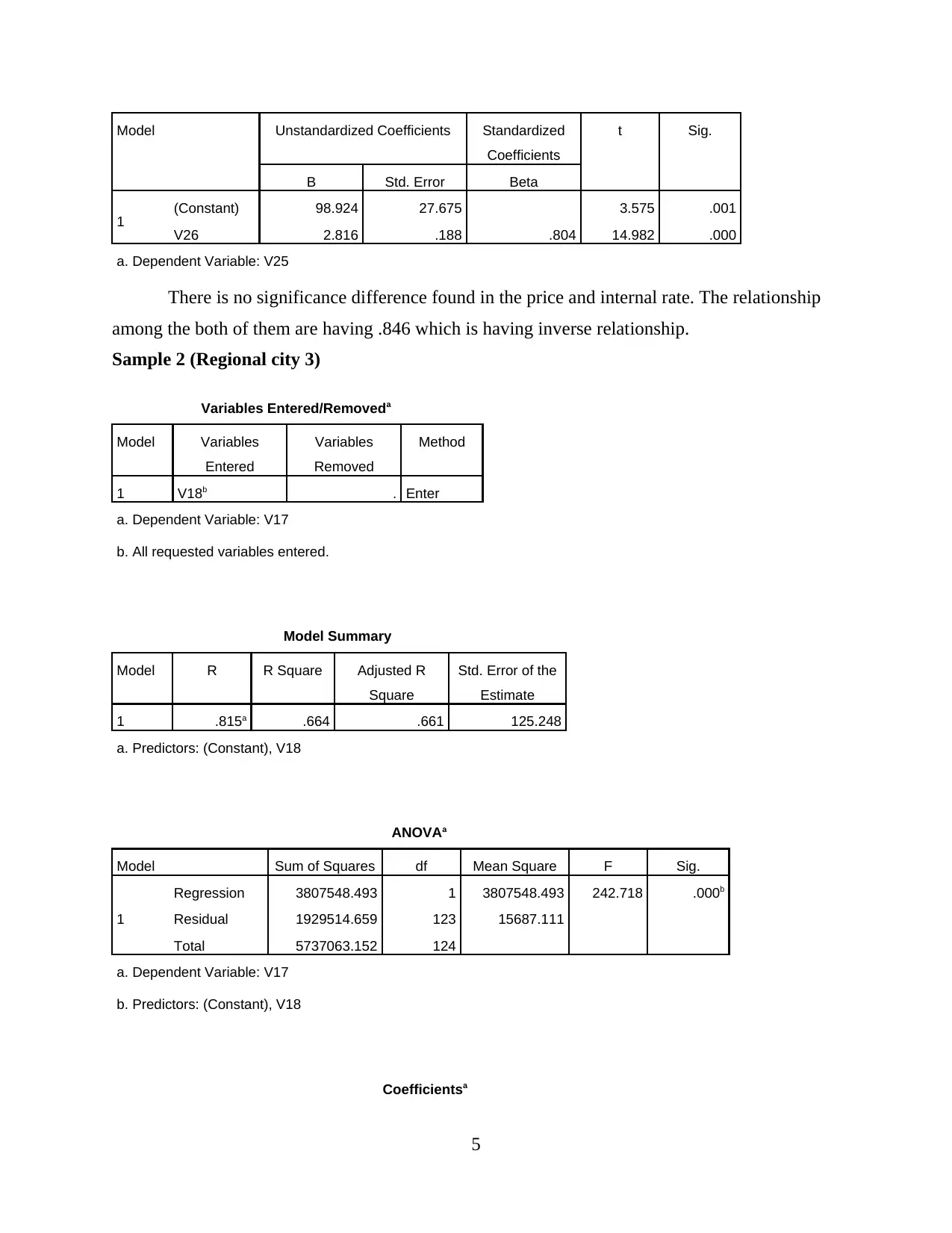
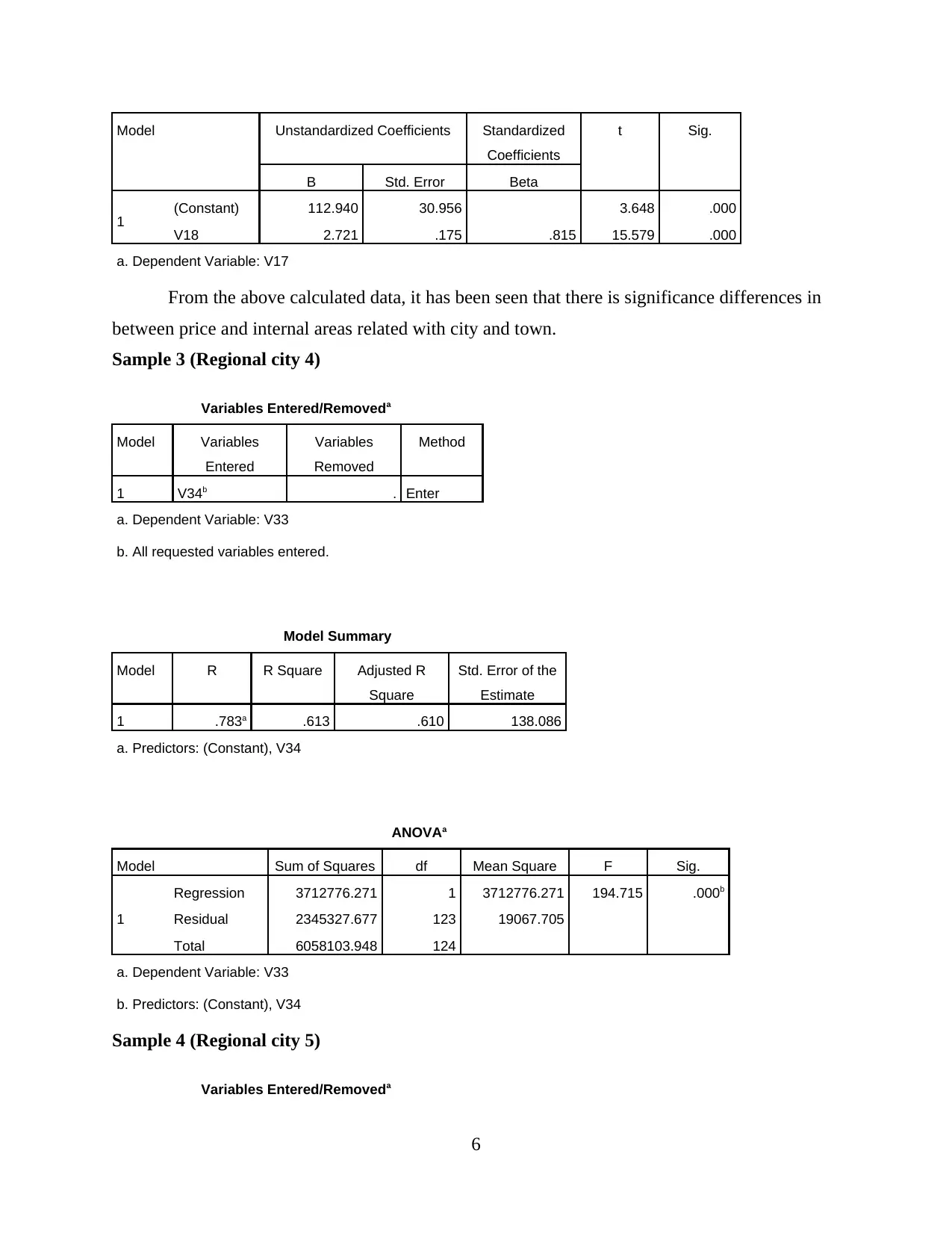
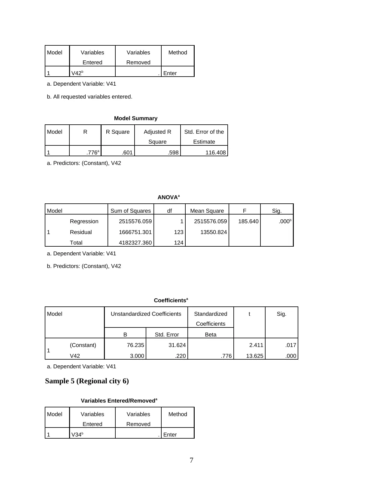
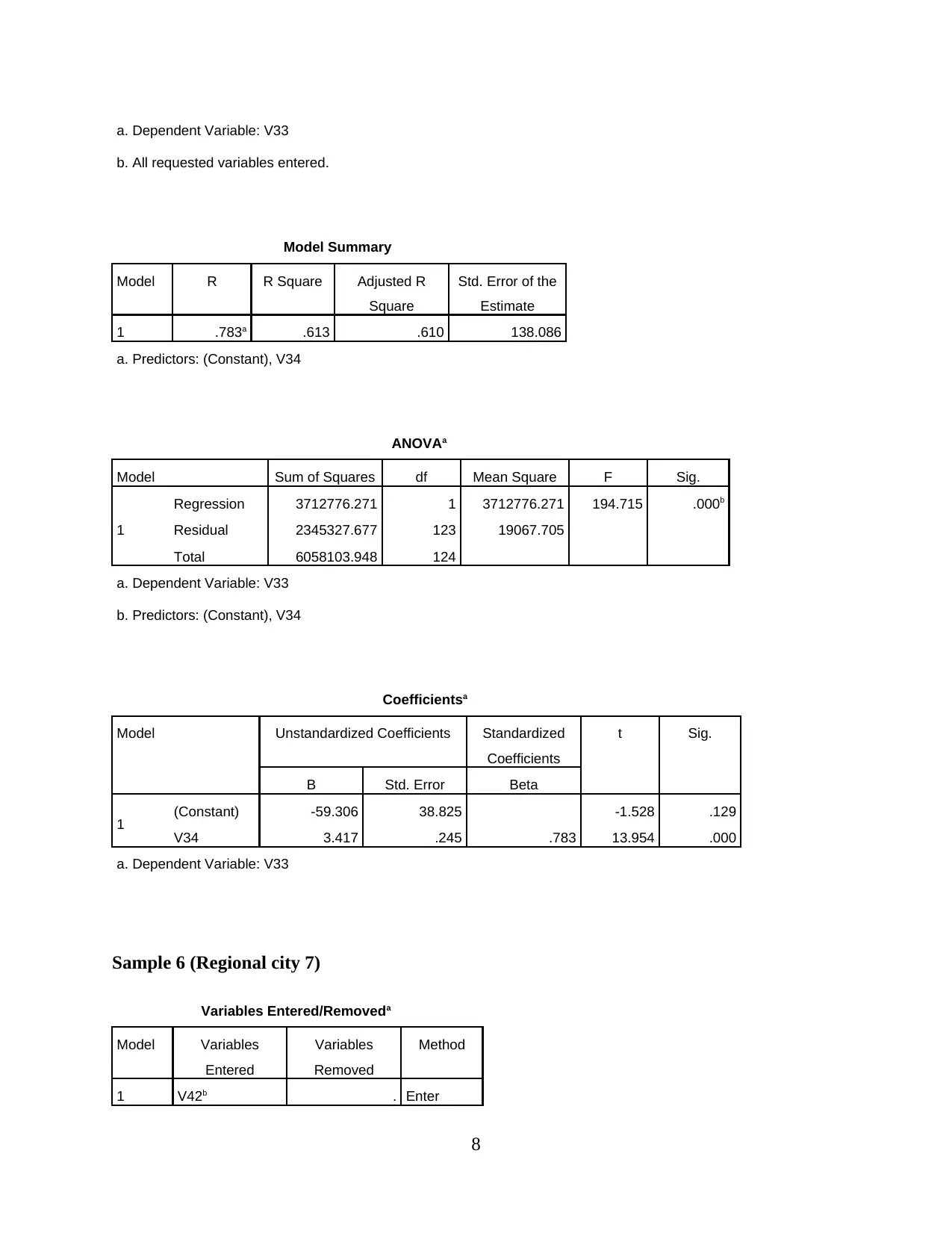
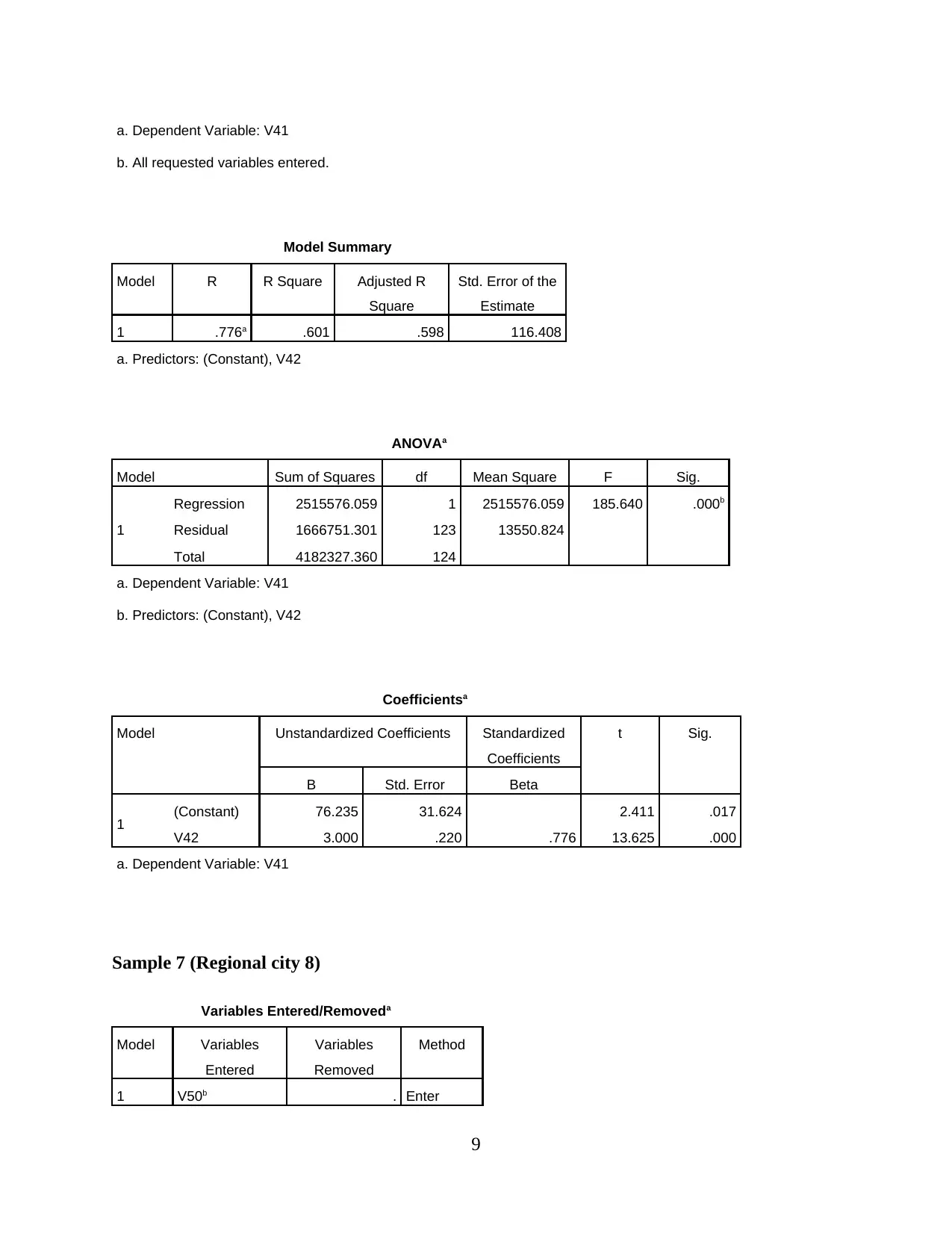
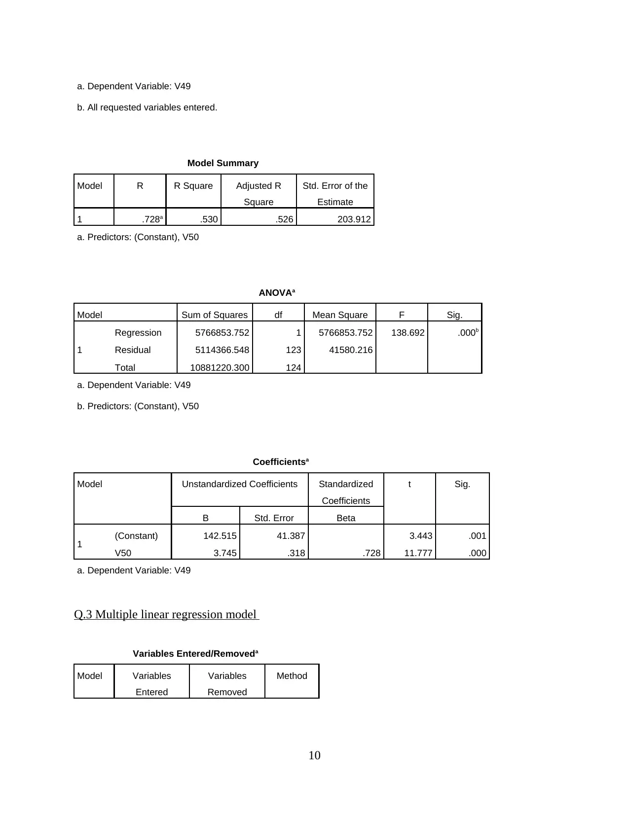
This report presents a statistical analysis of real estate market data, focusing on properties in non-capital cities and towns. The analysis utilizes data from various locations, employing statistical tools and techniques to derive meaningful insights. The report explores statistical inference, including case processing summaries and mean value calculations, to understand property price ranges. Furthermore, it delves into simple linear regression models for multiple regional cities, examining relationships between prices and internal areas. The report also includes multiple linear regression models, providing a comprehensive overview of the real estate market dynamics and highlighting significant differences in price and internal area relationships. The findings are supported by model summaries, ANOVA tables, and coefficient analyses, offering a detailed understanding of the factors influencing property values. The report provides a valuable resource for understanding the real estate market through statistical analysis.

STATISTICS

Table of Contents
INTRODUCTION...........................................................................................................................1
Q.1 Statistical inference topic.....................................................................................................1
Q.2 Simple linear regression model............................................................................................2
Q.3 Multiple linear regression model .......................................................................................10
CONCLUSION..............................................................................................................................11
REFERENCES..............................................................................................................................12

INTRODUCTION
According to this particular project which is related with real estate market in non-capital
cities and towns safe-as House real estate and wide national real national estate of the company.
The analysis is done from taking sample size and location with set price data from another town
and city. There are certain tools and techniques use for data analysis is being done in effective
manner.
Q.1 Statistical inference topic
Means
Case Processing Summary
Cases
Included Excluded Total
N Percent N Percent N Percent
V55 125 51.4% 118 48.6% 243 100.0%
V57 125 51.4% 118 48.6% 243 100.0%
Case Processing Summary
Cases
Included Excluded Total
N Percent N Percent N Percent
V55 125 51.4% 118 48.6% 243 100.0%
V57 125 51.4% 118 48.6% 243 100.0%
From the above analysis, it has been determine that total mean value of prices range of
samples A in accordance with the location of state for total number of 125 residential properties
for sale in each samples. By the help of reliable data analysis, it has been seen that there is 51.4%
of total average collected during the time.
Graph
1

Q.2 Simple linear regression model
Regression
Sample 0 (Regional city 1)
Model Summary
Model R R Square Adjusted R
Square
Std. Error of the
Estimate
1 .737a .543 .539 38.415
a. Predictors: (Constant), V9
Model Summary
2

Model R R Square Adjusted R
Square
Std. Error of the
Estimate
1 .737a .543 .539 38.415
a. Predictors: (Constant), V9
Coefficientsa
Model Unstandardized Coefficients Standardized
Coefficients
t Sig.
B Std. Error Beta
1 (Constant) 8.652 11.445 .756 .451
V9 .350 .029 .737 12.086 .000
a. Dependent Variable: V10
According to the above comparison is has been seen that .737 of regression which
would delivery appropriate outcomes during the time. Their is direct relationship among the
prices and internal areas. With the significant difference of .451 which is less than .5. There is no
any significant difference among both of them.
Sample 1 (Regional city 2)
Variables Entered/Removeda
Model Variables
Entered
Variables
Removed
Method
1 V9b . Enter
a. Dependent Variable: V10
b. All requested variables entered.
Model Summary
Model R R Square Adjusted R
Square
Std. Error of the
Estimate
1 .737a .543 .539 38.415
a. Predictors: (Constant), V9
ANOVAa
3

Model Sum of Squares df Mean Square F Sig.
1
Regression 215556.505 1 215556.505 146.070 .000b
Residual 181512.045 123 1475.708
Total 397068.550 124
a. Dependent Variable: V10
b. Predictors: (Constant), V9
Coefficientsa
Model Unstandardized Coefficients Standardized
Coefficients
t Sig.
B Std. Error Beta
1 (Constant) 8.652 11.445 .756 .451
V9 .350 .029 .737 12.086 .000
a. Dependent Variable: V10
Sample 2 (Regional city 3)
Variables Entered/Removeda
Model Variables
Entered
Variables
Removed
Method
1 V26b . Enter
a. Dependent Variable: V25
b. All requested variables entered.
Model Summary
Model R R Square Adjusted R
Square
Std. Error of the
Estimate
1 .804a .646 .643 116.705
a. Predictors: (Constant), V26
Coefficientsa
4

Model Unstandardized Coefficients Standardized
Coefficients
t Sig.
B Std. Error Beta
1 (Constant) 98.924 27.675 3.575 .001
V26 2.816 .188 .804 14.982 .000
a. Dependent Variable: V25
There is no significance difference found in the price and internal rate. The relationship
among the both of them are having .846 which is having inverse relationship.
Sample 2 (Regional city 3)
Variables Entered/Removeda
Model Variables
Entered
Variables
Removed
Method
1 V18b . Enter
a. Dependent Variable: V17
b. All requested variables entered.
Model Summary
Model R R Square Adjusted R
Square
Std. Error of the
Estimate
1 .815a .664 .661 125.248
a. Predictors: (Constant), V18
ANOVAa
Model Sum of Squares df Mean Square F Sig.
1
Regression 3807548.493 1 3807548.493 242.718 .000b
Residual 1929514.659 123 15687.111
Total 5737063.152 124
a. Dependent Variable: V17
b. Predictors: (Constant), V18
Coefficientsa
5

Model Unstandardized Coefficients Standardized
Coefficients
t Sig.
B Std. Error Beta
1 (Constant) 112.940 30.956 3.648 .000
V18 2.721 .175 .815 15.579 .000
a. Dependent Variable: V17
From the above calculated data, it has been seen that there is significance differences in
between price and internal areas related with city and town.
Sample 3 (Regional city 4)
Variables Entered/Removeda
Model Variables
Entered
Variables
Removed
Method
1 V34b . Enter
a. Dependent Variable: V33
b. All requested variables entered.
Model Summary
Model R R Square Adjusted R
Square
Std. Error of the
Estimate
1 .783a .613 .610 138.086
a. Predictors: (Constant), V34
ANOVAa
Model Sum of Squares df Mean Square F Sig.
1
Regression 3712776.271 1 3712776.271 194.715 .000b
Residual 2345327.677 123 19067.705
Total 6058103.948 124
a. Dependent Variable: V33
b. Predictors: (Constant), V34
Sample 4 (Regional city 5)
Variables Entered/Removeda
6

Model Variables
Entered
Variables
Removed
Method
1 V42b . Enter
a. Dependent Variable: V41
b. All requested variables entered.
Model Summary
Model R R Square Adjusted R
Square
Std. Error of the
Estimate
1 .776a .601 .598 116.408
a. Predictors: (Constant), V42
ANOVAa
Model Sum of Squares df Mean Square F Sig.
1
Regression 2515576.059 1 2515576.059 185.640 .000b
Residual 1666751.301 123 13550.824
Total 4182327.360 124
a. Dependent Variable: V41
b. Predictors: (Constant), V42
Coefficientsa
Model Unstandardized Coefficients Standardized
Coefficients
t Sig.
B Std. Error Beta
1 (Constant) 76.235 31.624 2.411 .017
V42 3.000 .220 .776 13.625 .000
a. Dependent Variable: V41
Sample 5 (Regional city 6)
Variables Entered/Removeda
Model Variables
Entered
Variables
Removed
Method
1 V34b . Enter
7

a. Dependent Variable: V33
b. All requested variables entered.
Model Summary
Model R R Square Adjusted R
Square
Std. Error of the
Estimate
1 .783a .613 .610 138.086
a. Predictors: (Constant), V34
ANOVAa
Model Sum of Squares df Mean Square F Sig.
1
Regression 3712776.271 1 3712776.271 194.715 .000b
Residual 2345327.677 123 19067.705
Total 6058103.948 124
a. Dependent Variable: V33
b. Predictors: (Constant), V34
Coefficientsa
Model Unstandardized Coefficients Standardized
Coefficients
t Sig.
B Std. Error Beta
1 (Constant) -59.306 38.825 -1.528 .129
V34 3.417 .245 .783 13.954 .000
a. Dependent Variable: V33
Sample 6 (Regional city 7)
Variables Entered/Removeda
Model Variables
Entered
Variables
Removed
Method
1 V42b . Enter
8

a. Dependent Variable: V41
b. All requested variables entered.
Model Summary
Model R R Square Adjusted R
Square
Std. Error of the
Estimate
1 .776a .601 .598 116.408
a. Predictors: (Constant), V42
ANOVAa
Model Sum of Squares df Mean Square F Sig.
1
Regression 2515576.059 1 2515576.059 185.640 .000b
Residual 1666751.301 123 13550.824
Total 4182327.360 124
a. Dependent Variable: V41
b. Predictors: (Constant), V42
Coefficientsa
Model Unstandardized Coefficients Standardized
Coefficients
t Sig.
B Std. Error Beta
1 (Constant) 76.235 31.624 2.411 .017
V42 3.000 .220 .776 13.625 .000
a. Dependent Variable: V41
Sample 7 (Regional city 8)
Variables Entered/Removeda
Model Variables
Entered
Variables
Removed
Method
1 V50b . Enter
9

a. Dependent Variable: V49
b. All requested variables entered.
Model Summary
Model R R Square Adjusted R
Square
Std. Error of the
Estimate
1 .728a .530 .526 203.912
a. Predictors: (Constant), V50
ANOVAa
Model Sum of Squares df Mean Square F Sig.
1
Regression 5766853.752 1 5766853.752 138.692 .000b
Residual 5114366.548 123 41580.216
Total 10881220.300 124
a. Dependent Variable: V49
b. Predictors: (Constant), V50
Coefficientsa
Model Unstandardized Coefficients Standardized
Coefficients
t Sig.
B Std. Error Beta
1 (Constant) 142.515 41.387 3.443 .001
V50 3.745 .318 .728 11.777 .000
a. Dependent Variable: V49
Q.3 Multiple linear regression model
Variables Entered/Removeda
Model Variables
Entered
Variables
Removed
Method
10

1
Type,
Bedrooms,
Internal Area
m^2b
. Enter
a. Dependent Variable: Price $000
b. All requested variables entered.
Model Summary
Model R R Square Adjusted R
Square
Std. Error of the
Estimate
1 .854a .729 .722 60.1528
a. Predictors: (Constant), Type, Bedrooms, Internal Area m^2
ANOVAa
Model Sum of Squares df Mean Square F Sig.
1
Regression 1177884.887 3 392628.296 108.510 .000b
Residual 437820.787 121 3618.354
Total 1615705.674 124
a. Dependent Variable: Price $000
b. Predictors: (Constant), Type, Bedrooms, Internal Area m^2
Coefficientsa
Model Unstandardized Coefficients Standardized
Coefficients
t Sig.
B Std. Error Beta
1
(Constant) -.522 44.110 -.012 .991
Internal Area m^2 2.720 .333 1.052 8.170 .000
Bedrooms -22.861 12.957 -.199 -1.764 .080
Type 7.385 16.761 .030 .441 .660
a. Dependent Variable: Price $000
11

CONCLUSION
From the above project report, it has been analyse that there are certain important aspects
that which are evaluated in this particular report. It has been determine that total number of
difference are providing appropriate outcomes to the researchers. It has been found that there is
direct relationship among various samples which is having certain kind of significant value and
reliability.
12