Case Study Analysis in Statistics

Student Name: Student ID: 1
Case Study Analysis in Statistics
Student Name: Student ID:
Unit Name: Unit ID:
Date Due: Professor Name:

Student Name: Student ID: 2
Acknowledgement

Student Name: Student ID: 3
Table of Contents
Acknowledgement...................................................................................................................................2
Answer 1..................................................................................................................................................4
Answer 2..................................................................................................................................................7
Answer 3..................................................................................................................................................9
Base model system................................................................................................................................10
B. Excel formula sheet for random cancelletion numbers.................................................................10
C. Hotel model solution for zero overbooked rooms.........................................................................12
D. Suggestions to the Hotel manager of hotel Heart Break...............................................................19
Answer 4................................................................................................................................................20
A. Regression model of Price on mileage travelled............................................................................20
Regression model of Price on Age of cars..............................................................................................21
Regression model of Price on Mileaage and Age of cars......................................................................22
Spearman’s Correlation between total mileage covered by cars and age of the cars..........................23
Answer 5................................................................................................................................................24
Model setup and solver solution...........................................................................................................24
Bibliography...............................................................................................................................................28

Student Name: Student ID: 4
Answer 1
A. Decision making is the game-plan picked by dissecting the assembled data about any
undertaking. The elective arrangements are additionally cross checked and choice tree
helps in building the whole model. There were a few stages associated with basic
leadership. At first the need of the choice and point of the task is examined. At that point
vital data is gathered and elective ways are recognized. The information was cross
checked and decision of definite option is finished. Organization executes the design and
the delayed consequences are recorded for future examination.
B. Alternate strategy is the following best arrangement acquired in choice displaying and is
known as option. Prospect hypothesis clarifies the elective procedure, for instance dread
of future misfortunes angers individuals more than the delight of future increases. In this
way, minimization of future failure is a contrasting option to boost the future additions.
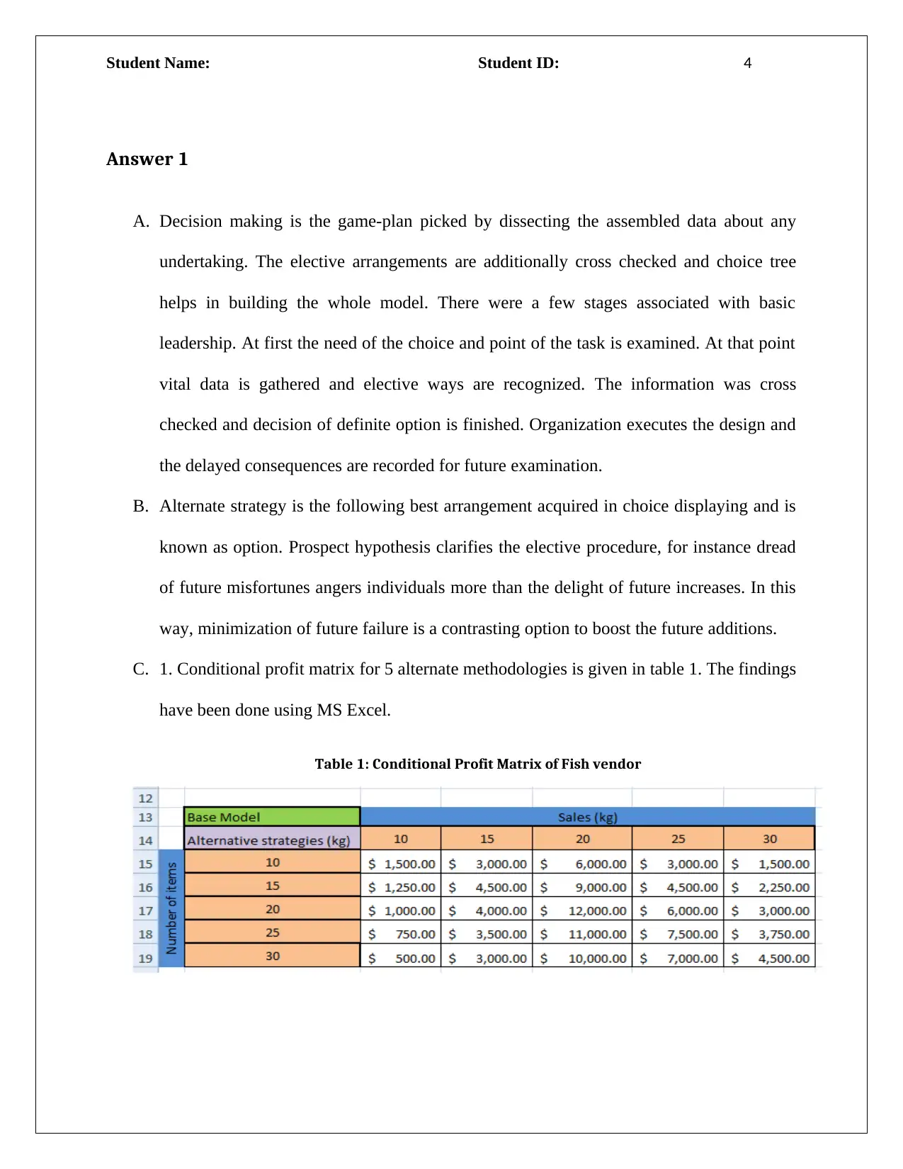
C. 1. Conditional profit matrix for 5 alternate methodologies is given in table 1. The findings
have been done using MS Excel.
Table 1: Conditional Profit Matrix of Fish vendor

Student Name: Student ID: 5
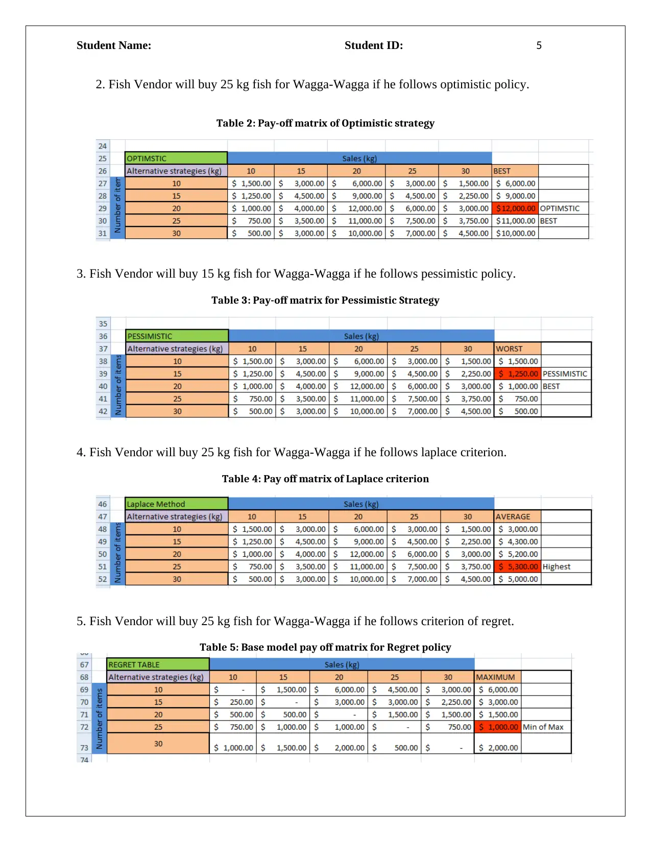
2. Fish Vendor will buy 25 kg fish for Wagga-Wagga if he follows optimistic policy.
Table 2: Pay-off matrix of Optimistic strategy
3. Fish Vendor will buy 15 kg fish for Wagga-Wagga if he follows pessimistic policy.
Table 3: Pay-off matrix for Pessimistic Strategy
4. Fish Vendor will buy 25 kg fish for Wagga-Wagga if he follows laplace criterion.
Table 4: Pay off matrix of Laplace criterion
5. Fish Vendor will buy 25 kg fish for Wagga-Wagga if he follows criterion of regret.
Table 5: Base model pay off matrix for Regret policy

Student Name: Student ID: 6
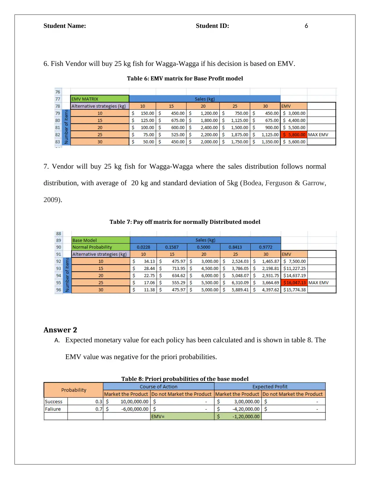
6. Fish Vendor will buy 25 kg fish for Wagga-Wagga if his decision is based on EMV.
Table 6: EMV matrix for Base Profit model
7. Vendor will buy 25 kg fish for Wagga-Wagga where the sales distribution follows normal
distribution, with average of 20 kg and standard deviation of 5kg (Bodea, Ferguson & Garrow,
2009).
Table 7: Pay off matrix for normally Distributed model
Answer 2
A. Expected monetary value for each policy has been calculated and is shown in table 8. The
EMV value was negative for the priori probabilities.
Table 8: Priori probabilities of the base model

Student Name: Student ID: 7
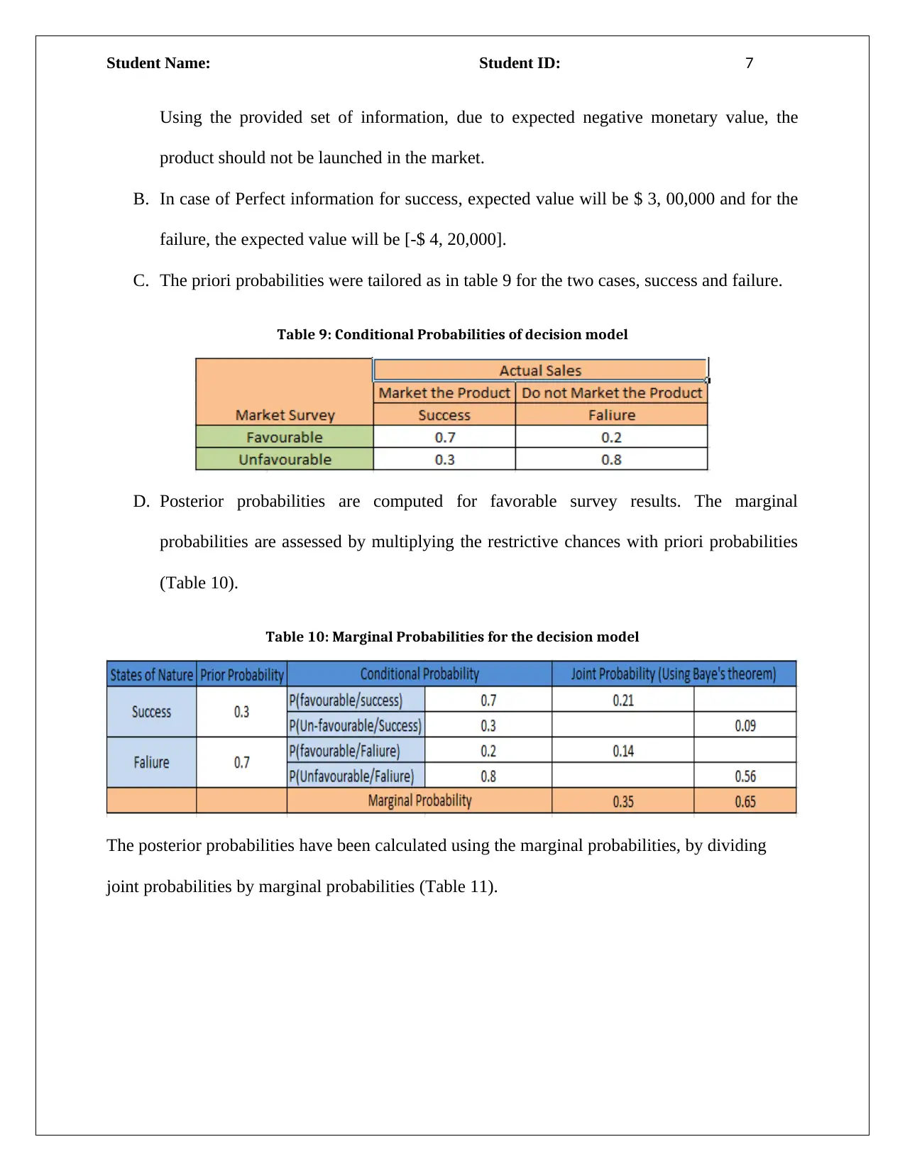
Using the provided set of information, due to expected negative monetary value, the
product should not be launched in the market.
B. In case of Perfect information for success, expected value will be $ 3, 00,000 and for the
failure, the expected value will be [-$ 4, 20,000].
C. The priori probabilities were tailored as in table 9 for the two cases, success and failure.
Table 9: Conditional Probabilities of decision model
D. Posterior probabilities are computed for favorable survey results. The marginal
probabilities are assessed by multiplying the restrictive chances with priori probabilities
(Table 10).
Table 10: Marginal Probabilities for the decision model
The posterior probabilities have been calculated using the marginal probabilities, by dividing
joint probabilities by marginal probabilities (Table 11).

Student Name: Student ID: 8
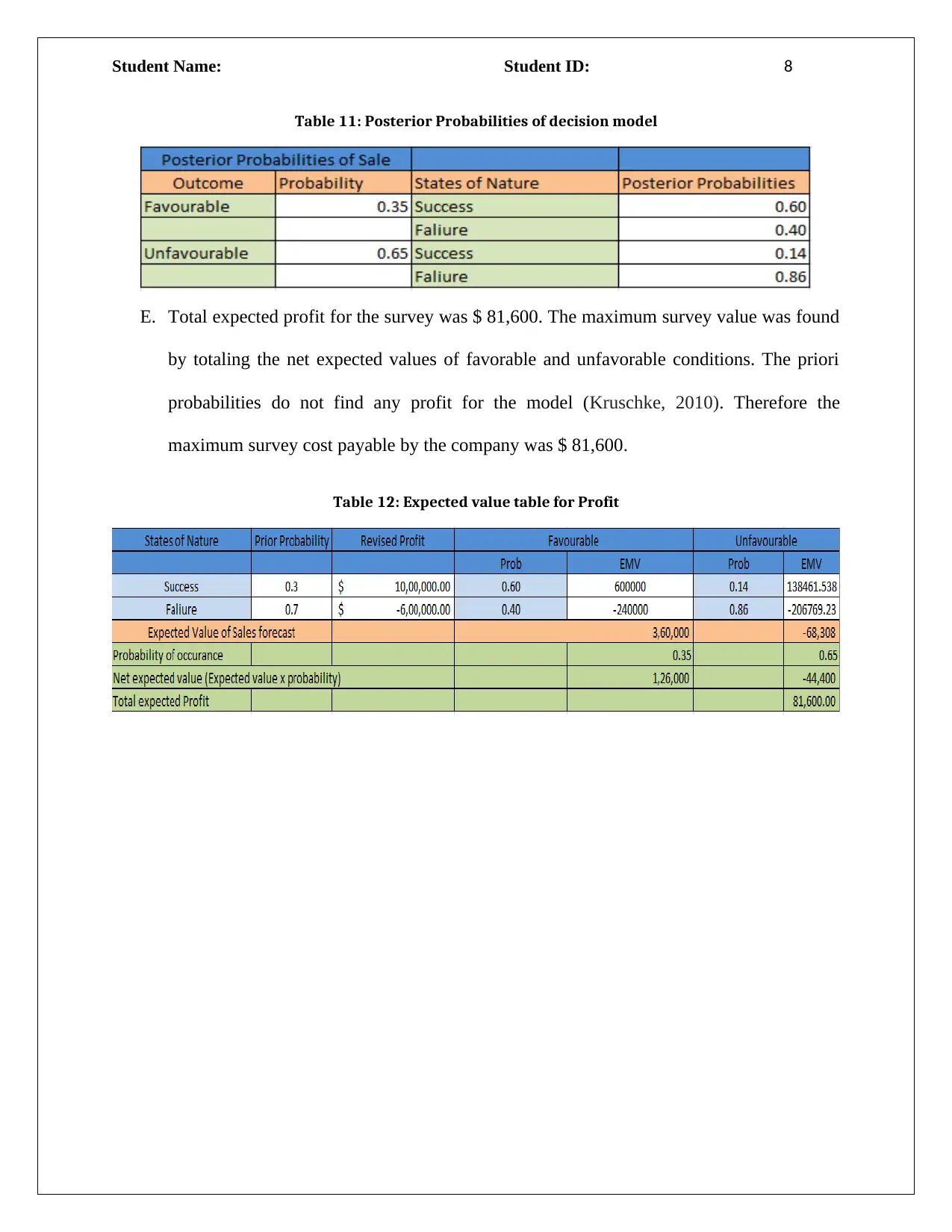
Table 11: Posterior Probabilities of decision model
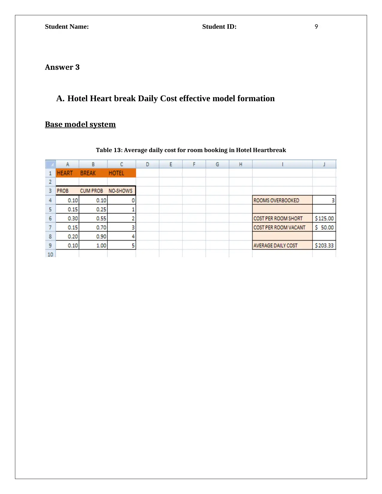
E. Total expected profit for the survey was $ 81,600. The maximum survey value was found
by totaling the net expected values of favorable and unfavorable conditions. The priori
probabilities do not find any profit for the model (Kruschke, 2010). Therefore the
maximum survey cost payable by the company was $ 81,600.
Table 12: Expected value table for Profit

Student Name: Student ID: 9
Answer 3
A. Hotel Heart break Daily Cost effective model formation
Base model system
Table 13: Average daily cost for room booking in Hotel Heartbreak

Student Name: Student ID: 10
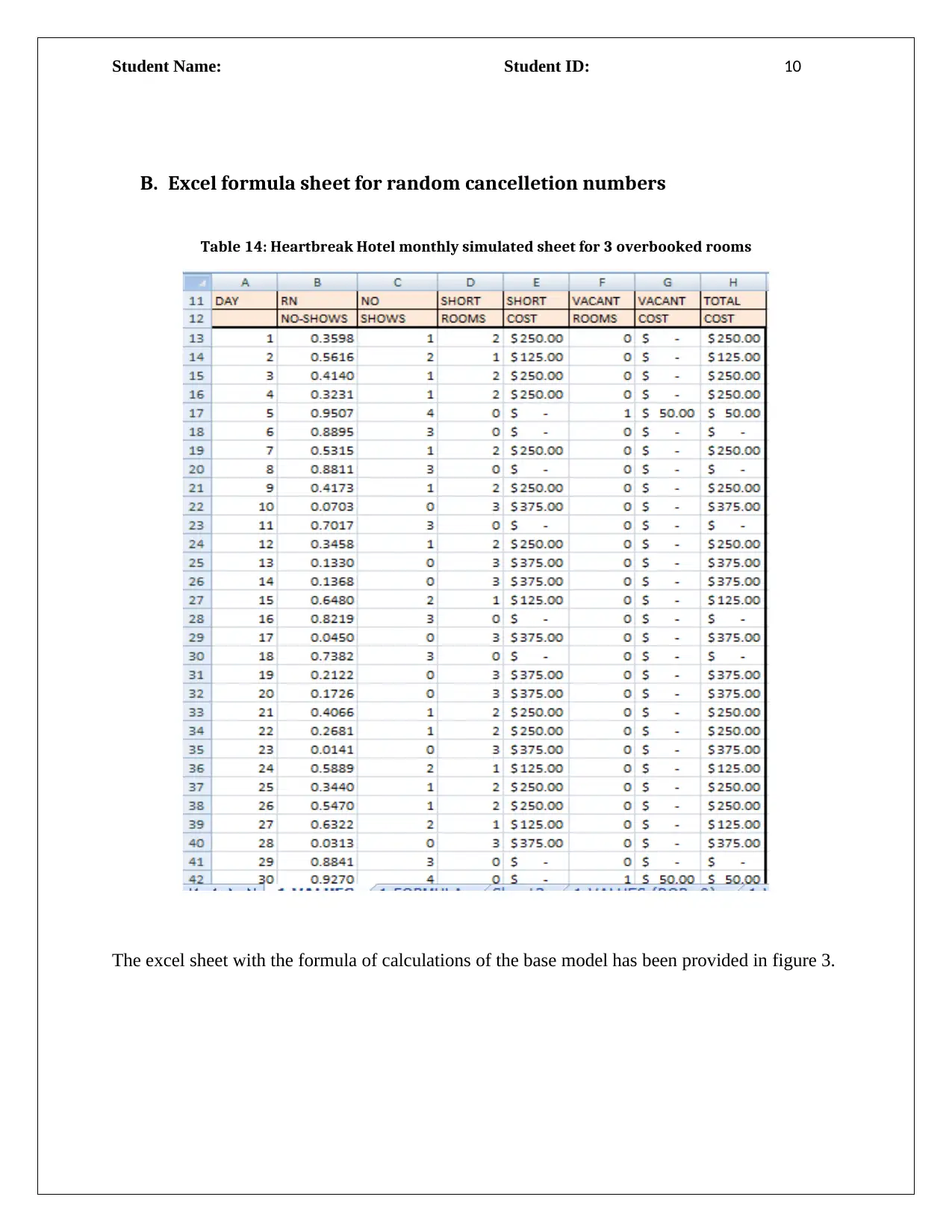
B. Excel formula sheet for random cancelletion numbers
Table 14: Heartbreak Hotel monthly simulated sheet for 3 overbooked rooms
The excel sheet with the formula of calculations of the base model has been provided in figure 3.

Student Name: Student ID: 11
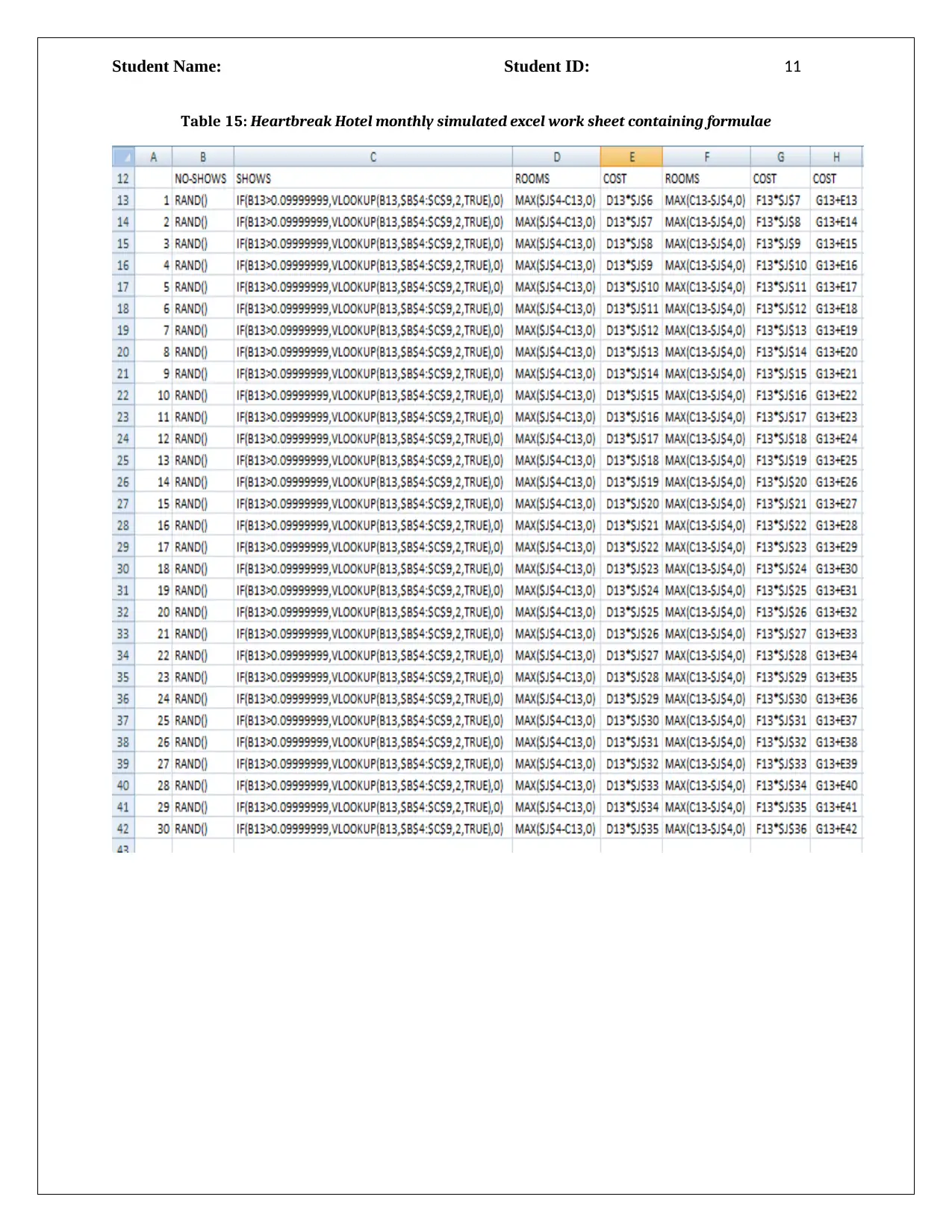
Table 15: Heartbreak Hotel monthly simulated excel work sheet containing formulae

Student Name: Student ID: 12
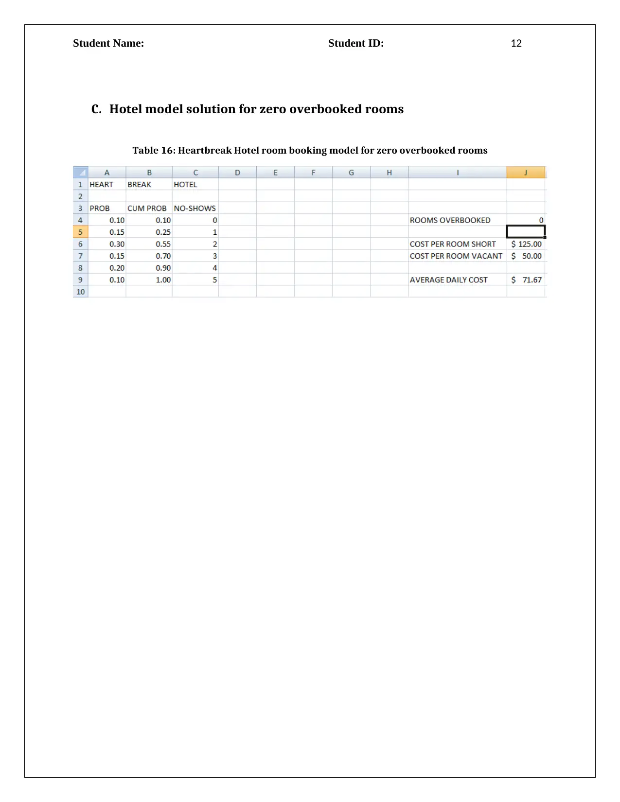
C. Hotel model solution for zero overbooked rooms
Table 16: Heartbreak Hotel room booking model for zero overbooked rooms

Student Name: Student ID: 13
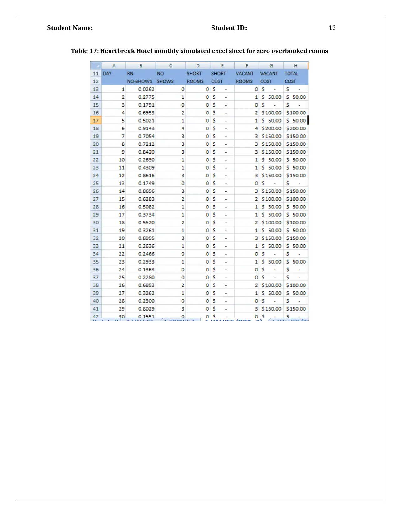
Table 17: Heartbreak Hotel monthly simulated excel sheet for zero overbooked rooms

Student Name: Student ID: 14
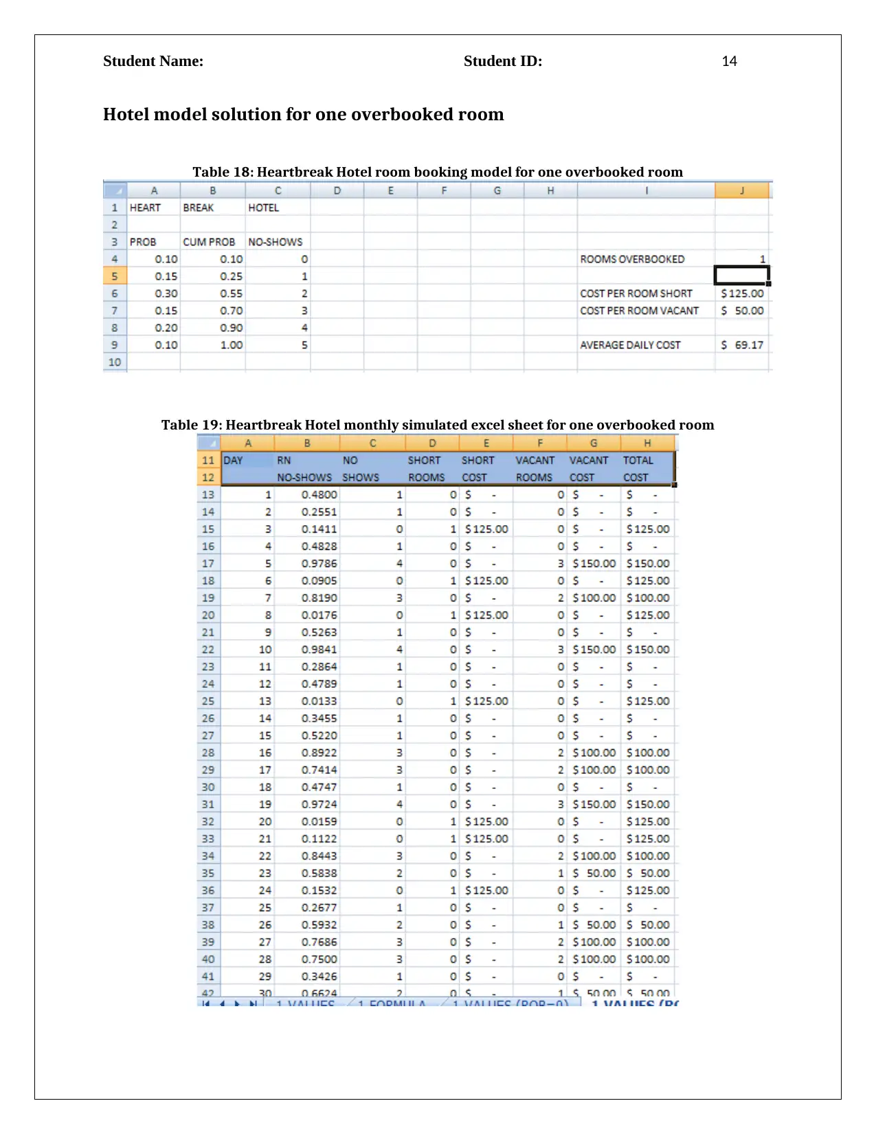
Hotel model solution for one overbooked room
Table 18: Heartbreak Hotel room booking model for one overbooked room
Table 19: Heartbreak Hotel monthly simulated excel sheet for one overbooked room

Student Name: Student ID: 15
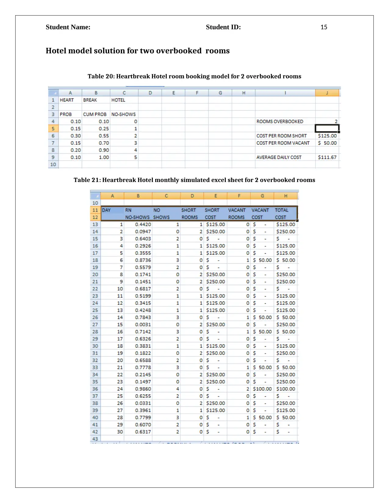
Hotel model solution for two overbooked rooms
Table 20: Heartbreak Hotel room booking model for 2 overbooked rooms
Table 21: Heartbreak Hotel monthly simulated excel sheet for 2 overbooked rooms

Student Name: Student ID: 16
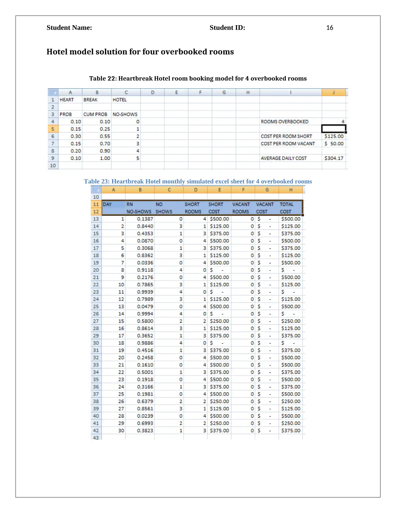
Hotel model solution for four overbooked rooms
Table 22: Heartbreak Hotel room booking model for 4 overbooked rooms
Table 23: Heartbreak Hotel monthly simulated excel sheet for 4 overbooked rooms

Student Name: Student ID: 17
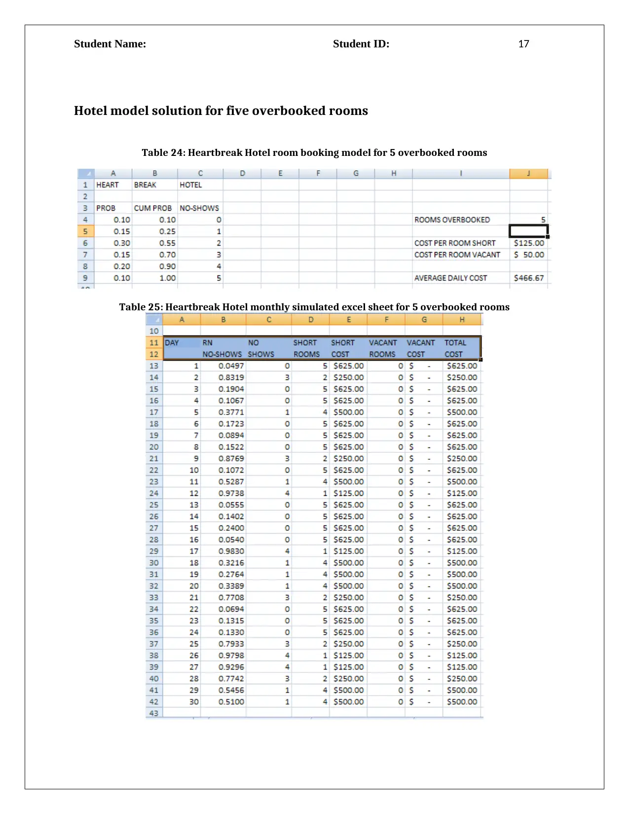
Hotel model solution for five overbooked rooms
Table 24: Heartbreak Hotel room booking model for 5 overbooked rooms
Table 25: Heartbreak Hotel monthly simulated excel sheet for 5 overbooked rooms

Student Name: Student ID: 18
D. Suggestions to the Hotel manager of hotel Heart Break
To 8th May 2018
The manager
Hotel Heart Break
Synopsis on Average daily cost and Overbooking of rooms
The reenacted normal day by day cost of the Heart Break inn was $ 203.33. Number of
overbooked rooms was at first thought to be three. Normal no shows by clients was in the
vicinity of zero and five, every day. The month to month information for every day cost
was computed by picking the no shows of the clients in an irregular example from the
rundown of no shows. The adjustment in normal day by day cost for the clients was
noted. An exceed expectations spreadsheet was made to analyze the result of no shows on
the day by day normal cost. The normal every day cost of the inn was re-ascertained and
noted by changing the quantity of overbooked rooms in the inn. The normal day by day
cost was computed for five unique estimations of no shows of clients. It was uncovered
that the day by day normal cost lessened when the quantity of overbooked rooms in the
hotel was diminished (Zakhary et al., 2011). The base recreated normal every day cost
was observed to be $ 69.17 for one overbooked room. Henceforth diminishing number of
overbooked rooms was beneficial for the hotel (Yang, Pan & Song, 2014).
Sincerely Yours
__________________

Student Name: Student ID: 19
Answer 4
A. Regression model of Price on mileage travelled
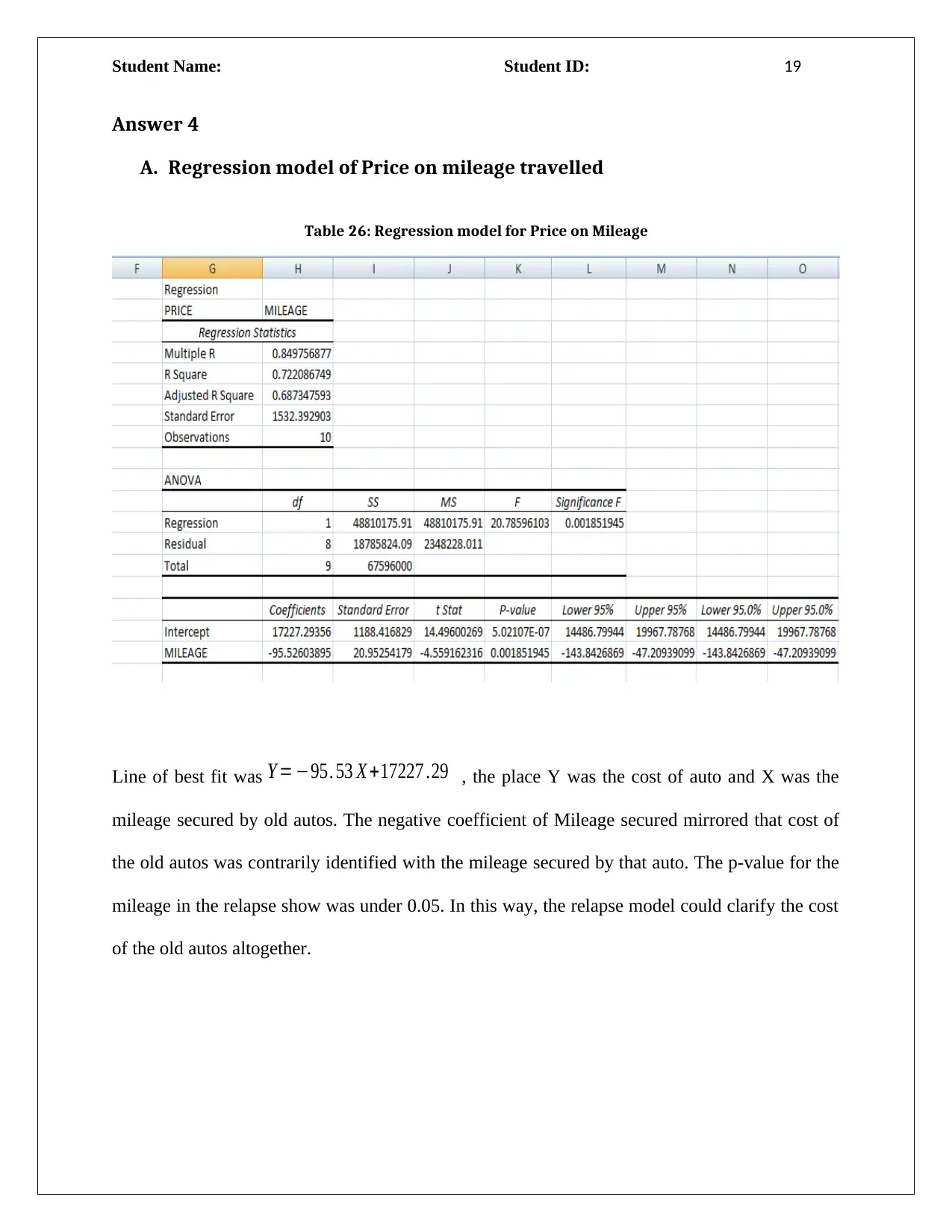
Table 26: Regression model for Price on Mileage
Line of best fit was Y = −95. 53 X +17227 .29 , the place Y was the cost of auto and X was the
mileage secured by old autos. The negative coefficient of Mileage secured mirrored that cost of
the old autos was contrarily identified with the mileage secured by that auto. The p-value for the
mileage in the relapse show was under 0.05. In this way, the relapse model could clarify the cost
of the old autos altogether.

Student Name: Student ID: 20
Regression model of Price on Age of cars
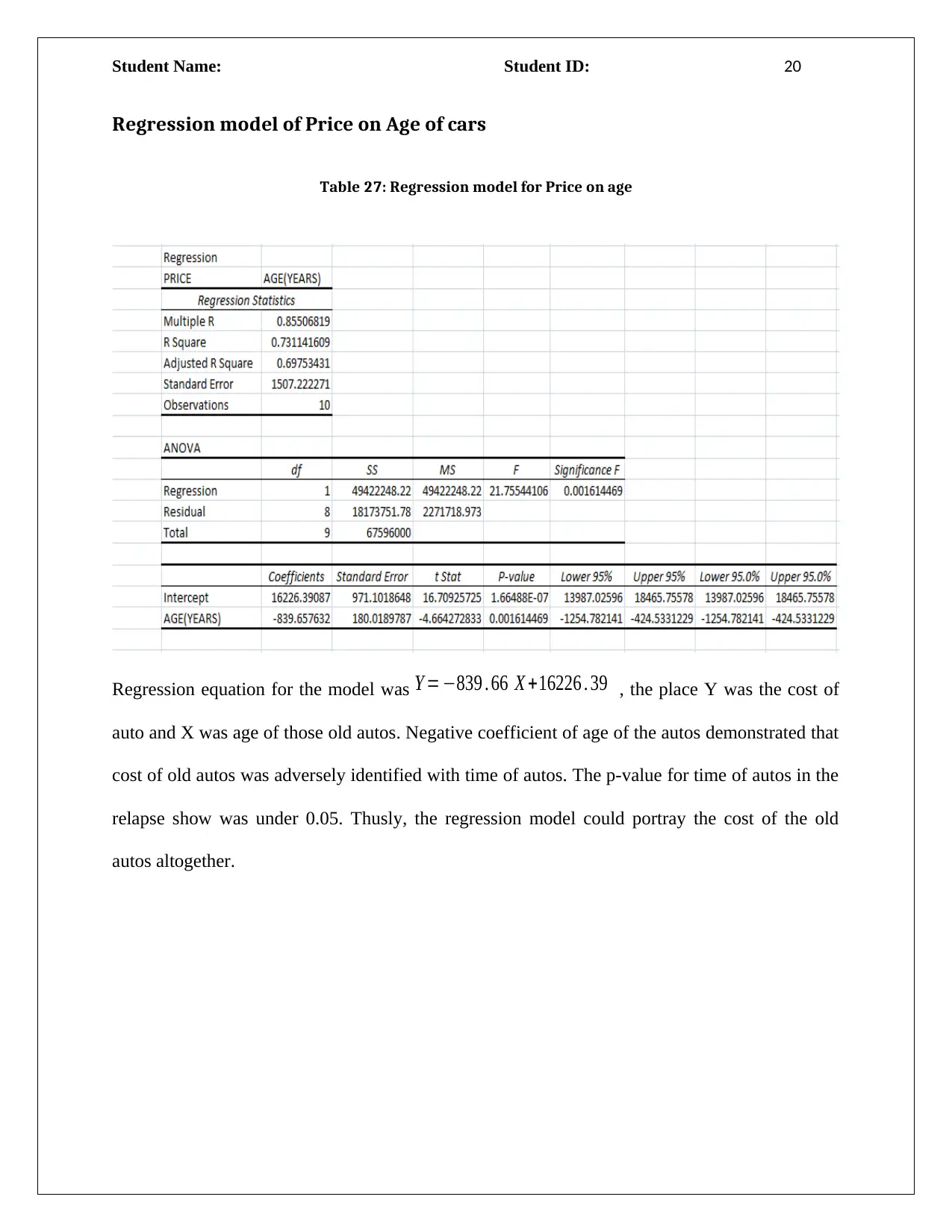
Table 27: Regression model for Price on age
Regression equation for the model was Y = −839 . 66 X +16226 . 39 , the place Y was the cost of
auto and X was age of those old autos. Negative coefficient of age of the autos demonstrated that
cost of old autos was adversely identified with time of autos. The p-value for time of autos in the
relapse show was under 0.05. Thusly, the regression model could portray the cost of the old
autos altogether.

Student Name: Student ID: 21
Regression model of Price on Mileaage and Age of cars
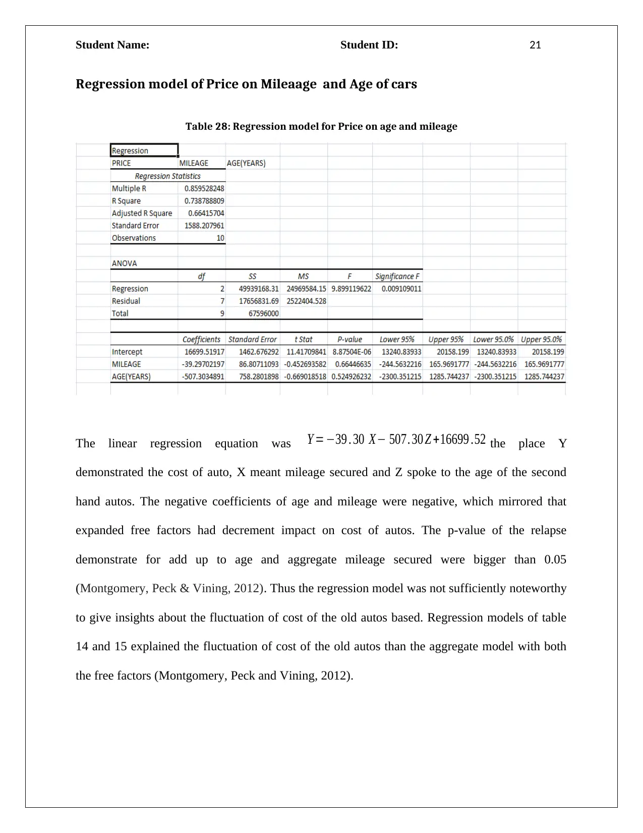
Table 28: Regression model for Price on age and mileage
The linear regression equation was Y = −39 . 30 X− 507. 30 Z +16699 .52 the place Y
demonstrated the cost of auto, X meant mileage secured and Z spoke to the age of the second
hand autos. The negative coefficients of age and mileage were negative, which mirrored that
expanded free factors had decrement impact on cost of autos. The p-value of the relapse
demonstrate for add up to age and aggregate mileage secured were bigger than 0.05
(Montgomery, Peck & Vining, 2012). Thus the regression model was not sufficiently noteworthy
to give insights about the fluctuation of cost of the old autos based. Regression models of table
14 and 15 explained the fluctuation of cost of the old autos than the aggregate model with both
the free factors (Montgomery, Peck and Vining, 2012).

Student Name: Student ID: 22
b. Singular models performed superior to anything the aggregate regression model. The adjusted
R-square estimation of mileage-value display was 73.11% which clarified the fluctuation of cost
in the second model. The significance values of intercept and mileage at the auto cost and
aggregate mileage demonstrate were likewise under 0.05. Regression coefficients of auto age and
aggregate mileage secured demonstrated that cost of the old autos was adversely identified with
the clarifying components. The connection nature between cost of old autos and aggregate
mileage secured, time of old auto was clear because of evident realities (Seber, & Lee, 2012).
c.
Spearman’s Correlation between total mileage covered by cars and age of the
cars
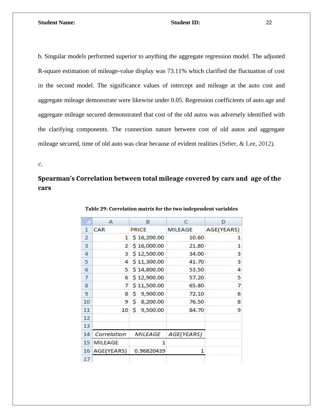
Table 29: Correlation matrix for the two independent variables

Student Name: Student ID: 23
Add up to mileage voyaged and age of an old auto was positively associated. The correlation was
essentially high in nature. The model with the two free factors was legitimate in nature, obvious
from the connection score. Total mileage secured by the old auto was the better free factor,
which was obvious from the relapse demonstrate. Both the factors were similarly vital in
choosing cost of autos.
Answer 5
Model setup and solver solution
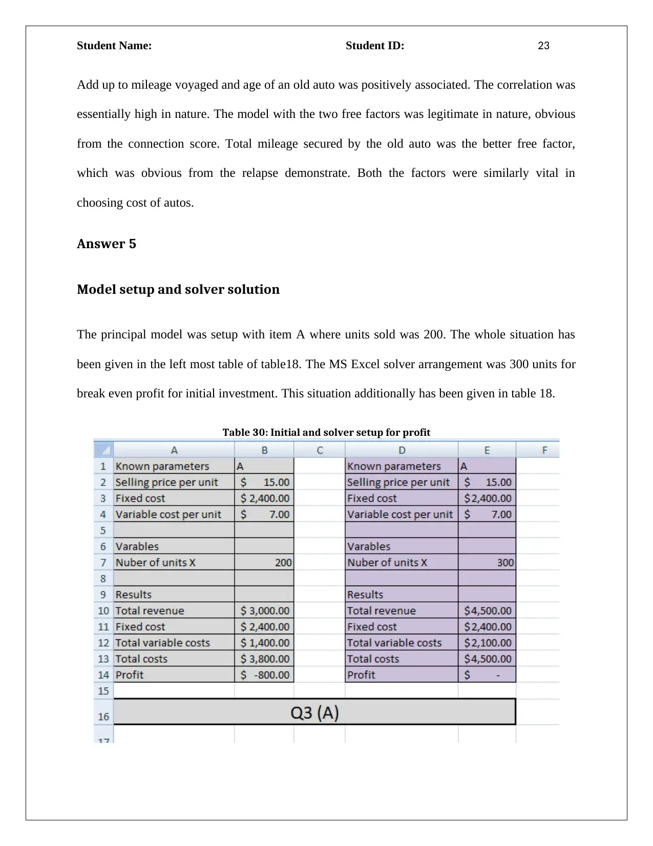
The principal model was setup with item A where units sold was 200. The whole situation has
been given in the left most table of table18. The MS Excel solver arrangement was 300 units for
break even profit for initial investment. This situation additionally has been given in table 18.
Table 30: Initial and solver setup for profit

Student Name: Student ID: 24
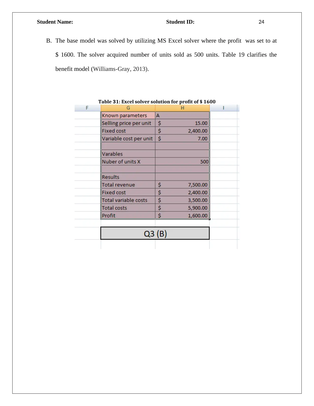
B. The base model was solved by utilizing MS Excel solver where the profit was set to at
$ 1600. The solver acquired number of units sold as 500 units. Table 19 clarifies the
benefit model (Williams-Gray, 2013).
Table 31: Excel solver solution for profit of $ 1600

Student Name: Student ID: 25
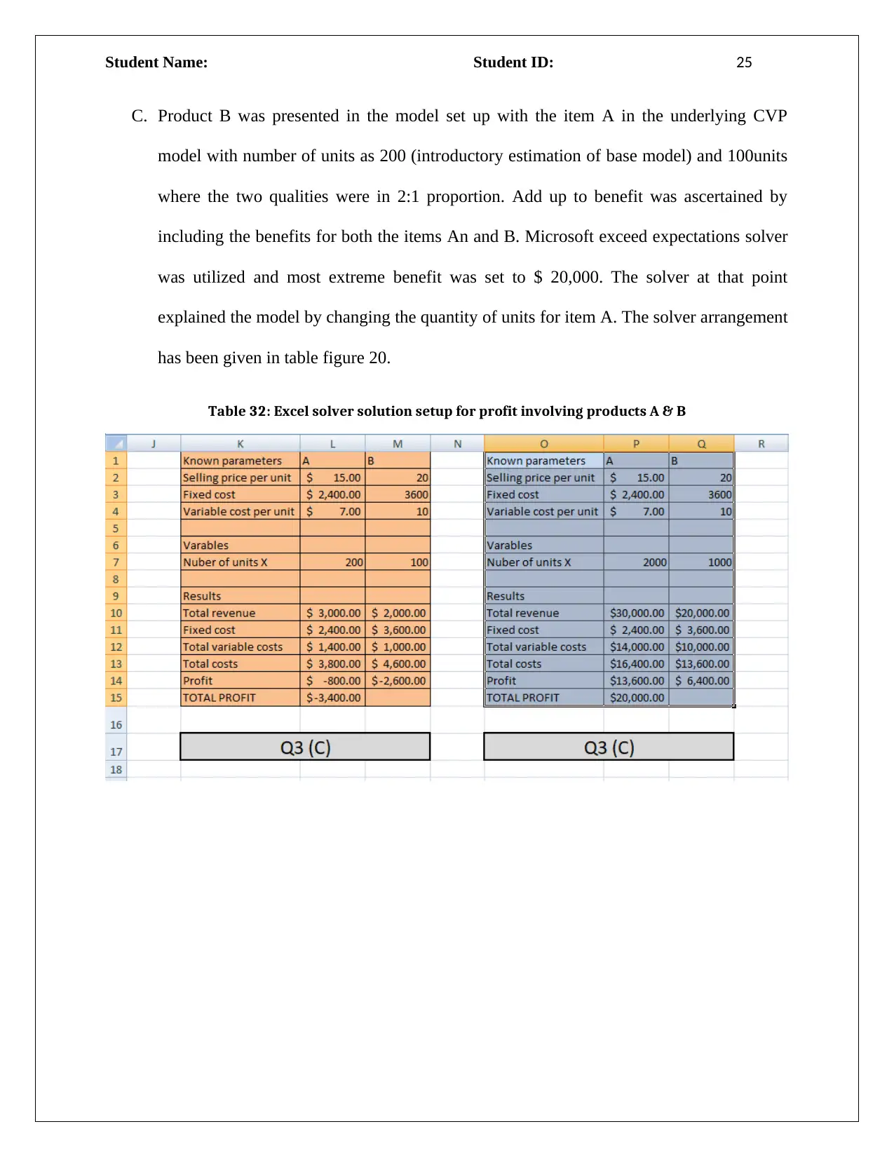
C. Product B was presented in the model set up with the item A in the underlying CVP
model with number of units as 200 (introductory estimation of base model) and 100units
where the two qualities were in 2:1 proportion. Add up to benefit was ascertained by
including the benefits for both the items An and B. Microsoft exceed expectations solver
was utilized and most extreme benefit was set to $ 20,000. The solver at that point
explained the model by changing the quantity of units for item A. The solver arrangement
has been given in table figure 20.
Table 32: Excel solver solution setup for profit involving products A & B

Student Name: Student ID: 26
Bibliography
Bodea, T., Ferguson, M., & Garrow, L. (2009). Data set—choice-based revenue management:
Data from a major hotel chain. Manufacturing & Service Operations Management, 11(2),
356-361.
Kruschke, J. K. (2010). What to believe: Bayesian methods for data analysis. Trends in cognitive
sciences, 14(7), 293-300.
Montgomery, D. C., Peck, E. A., & Vining, G. G. (2012). Introduction to linear regression
analysis (Vol. 821). John Wiley & Sons.
Seber, G. A., & Lee, A. J. (2012). Linear regression analysis (Vol. 329). John Wiley & Sons.
Williams-Gray, C. H., Mason, S. L., Evans, J. R., Foltynie, T., Brayne, C., Robbins, T. W., &
Barker, R. A. (2013). The CamPaIGN study of Parkinson's disease: 10-year outlook in an
incident population-based cohort. J Neurol Neurosurg Psychiatry, 84(11), 1258-1264.
Yang, Y., Pan, B., & Song, H. (2014). Predicting hotel demand using destination marketing
organization’s web traffic data. Journal of Travel Research, 53(4), 433-447.
Zakhary, A., Atiya, A. F., El-Shishiny, H., & Gayar, N. E. (2011). Forecasting hotel arrivals and
occupancy using Monte Carlo simulation. Journal of Revenue and Pricing
Management, 10(4), 344-366.