Chemical Reactor Control System Design

The assignment focuses on designing and simulating a proportional (P) controller for a chemical reactor. It involves determining system parameters, implementing the controller using MATLAB, and analyzing its performance through step response plots. The simulation considers constraints on the control signal and explores the impact of 80% input limitations on the closed-loop system's behavior.

Real Time Estimation and Control
Question 1:
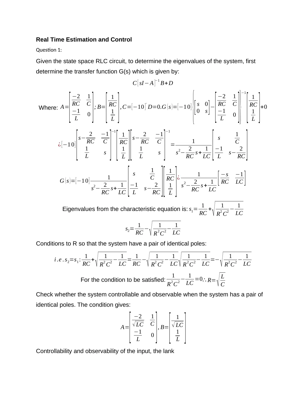
Given the state space RLC circuit, to determine the eigenvalues of the system, first
determine the transfer function G(s) which is given by:
C [ sI− A ]
−1 B+ D
Where: A=
[ −2
RC
1
C
−1
L 0 ]; B=
[ 1
RC
1
L ], C= [−10 ]' D=0. G ( s ) = [ −1 0 ]
{[ s 0
0 s ] −
[ −2
RC
1
C
−1
L 0 ] }
−1
[ 1
RC
1
L ] +0
¿ [−1 0 ]
[s− 2
RC
−1
C
1
L s ]−1
[ 1
RC
1
L ] [s− 2
RC
−1
C
1
L s ]−1
= 1
s2− 2
RC s + 1
LC [ s 1
C
−1
L s− 2
RC ]
G ( s ) = [ −1 0 ] 1
s2− 2
RC s+ 1
LC [ s 1
C
−1
L s− 2
RC ] [ 1
RC
1
L ]¿ 1
s2− 2
RC s + 1
LC
[ −s
RC
−1
LC ]
Eigenvalues from the characteristic equation is: s1= 1
RC + √ 1
R2 C2 − 1
LC
s2= 1
RC − √ 1
R2 C2 − 1
LC
Conditions to R so that the system have a pair of identical poles:
i .e . s2=s1 : 1
RC + √ 1
R2 C2 − 1
LC = 1
RC − √ 1
R2 C2 − 1
LC √ 1
R2 C2 − 1
LC =− √ 1
R2 C2 − 1
LC
For the condition to be satisfied: 1
R2 C2 − 1
LC =0∴ R= √ L
C
Check whether the system controllable and observable when the system has a pair of
identical poles. The condition gives:
A=
[ −2
√ LC
1
C
−1
L 0 ], B=
[ 1
√ LC
1
L ]Controllability and observability of the input, the lank

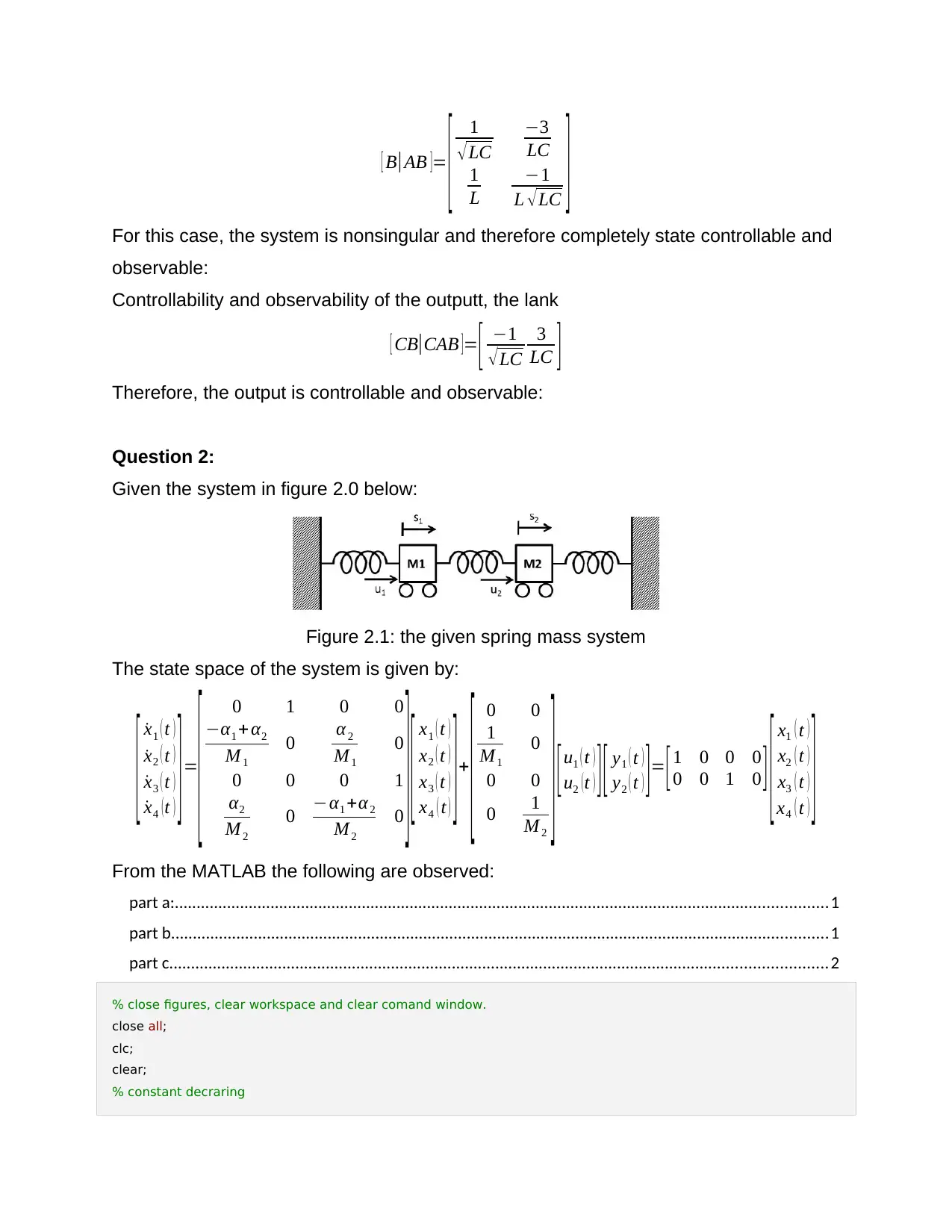
[ B|AB ]=
[ 1
√LC
−3
LC
1
L
−1
L √LC ]For this case, the system is nonsingular and therefore completely state controllable and
observable:
Controllability and observability of the outputt, the lank
[ CB|CAB ]= [ −1
√ LC
3
LC ]
Therefore, the output is controllable and observable:
Question 2:
Given the system in figure 2.0 below:
Figure 2.1: the given spring mass system
The state space of the system is given by:
[ ˙x1 ( t )
˙x2 ( t )
˙x3 ( t )
˙x4 ( t ) ] =
[ 0 1 0 0
−α1 +α2
M 1
0 α 2
M1
0
0 0 0 1
α2
M 2
0 −α1 +α 2
M2
0 ] [ x1 ( t )
x2 ( t )
x3 ( t )
x4 ( t ) ] +
[ 0 0
1
M1
0
0 0
0 1
M2
] [ u1 ( t )
u2 ( t ) ] [ y1 ( t )
y2 ( t ) ]= [1 0 0 0
0 0 1 0 ] [ x1 ( t )
x2 ( t )
x3 ( t )
x4 ( t ) ]
From the MATLAB the following are observed:
part a:......................................................................................................................................................1
part b.......................................................................................................................................................1
part c.......................................................................................................................................................2
% close figures, clear workspace and clear comand window.
close all;
clc;
clear;
% constant decraring

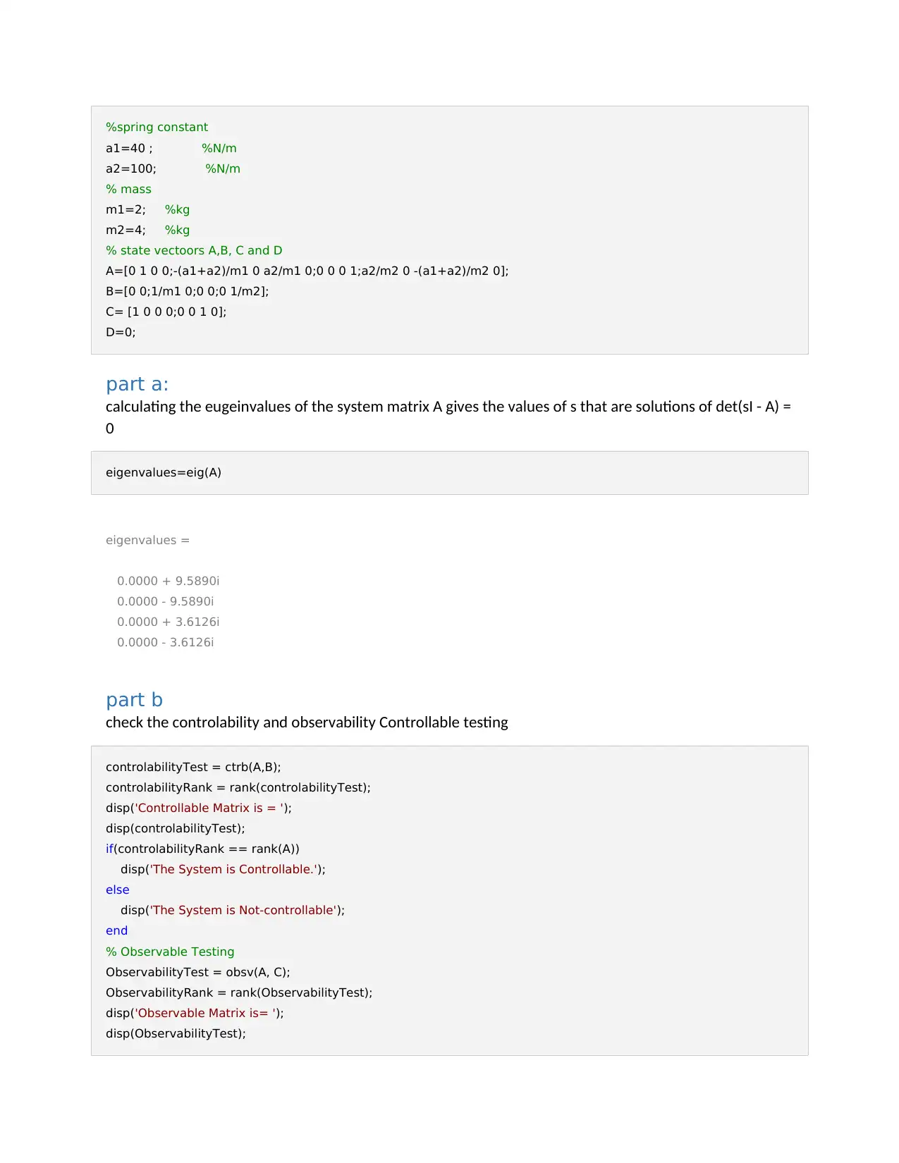
%spring constant
a1=40 ; %N/m
a2=100; %N/m
% mass
m1=2; %kg
m2=4; %kg
% state vectoors A,B, C and D
A=[0 1 0 0;-(a1+a2)/m1 0 a2/m1 0;0 0 0 1;a2/m2 0 -(a1+a2)/m2 0];
B=[0 0;1/m1 0;0 0;0 1/m2];
C= [1 0 0 0;0 0 1 0];
D=0;
part a:
calculating the eugeinvalues of the system matrix A gives the values of s that are solutions of det(sI - A) =
0
eigenvalues=eig(A)
eigenvalues =
0.0000 + 9.5890i
0.0000 - 9.5890i
0.0000 + 3.6126i
0.0000 - 3.6126i
part b
check the controlability and observability Controllable testing
controlabilityTest = ctrb(A,B);
controlabilityRank = rank(controlabilityTest);
disp('Controllable Matrix is = ');
disp(controlabilityTest);
if(controlabilityRank == rank(A))
disp('The System is Controllable.');
else
disp('The System is Not-controllable');
end
% Observable Testing
ObservabilityTest = obsv(A, C);
ObservabilityRank = rank(ObservabilityTest);
disp('Observable Matrix is= ');
disp(ObservabilityTest);

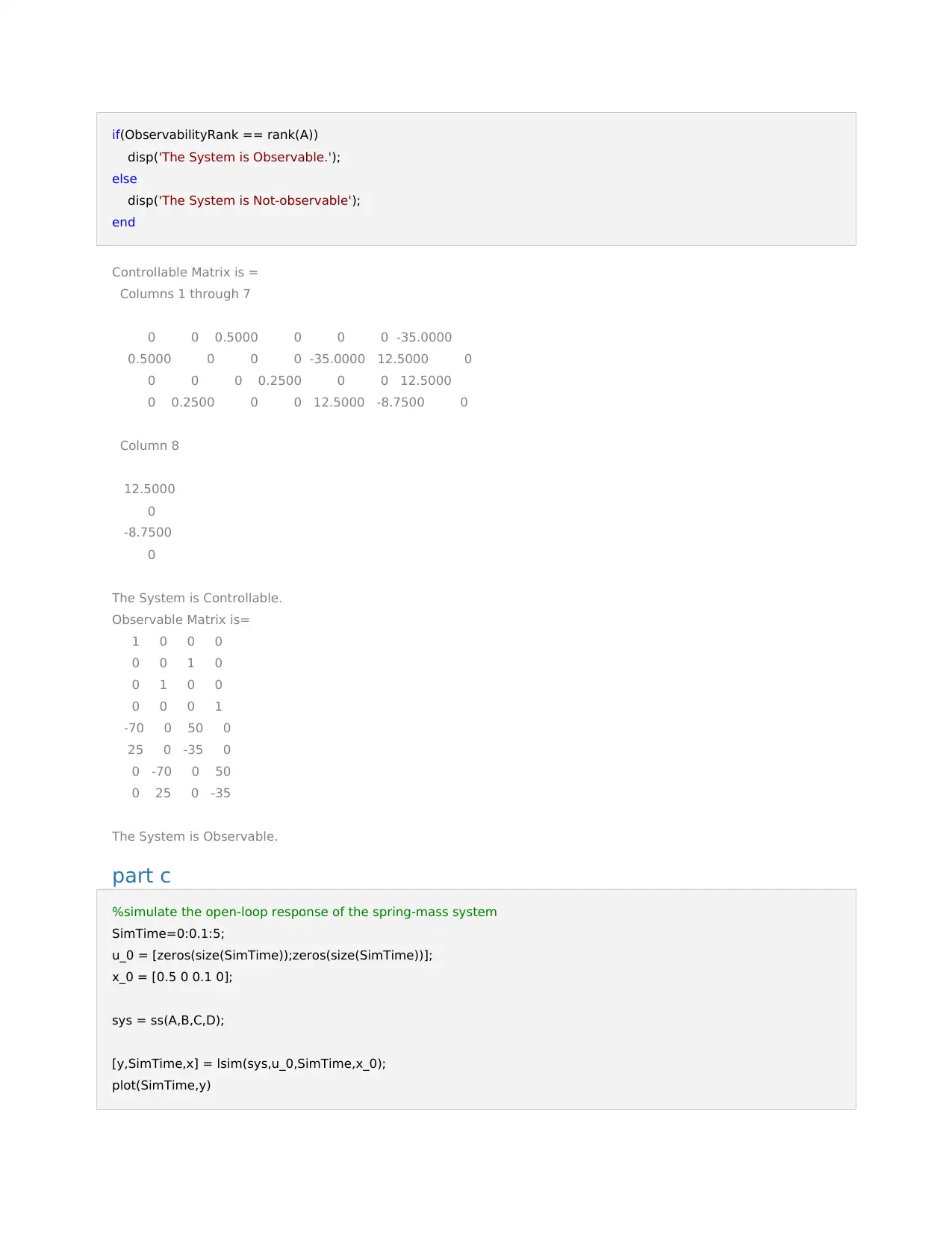
if(ObservabilityRank == rank(A))
disp('The System is Observable.');
else
disp('The System is Not-observable');
end
Controllable Matrix is =
Columns 1 through 7
0 0 0.5000 0 0 0 -35.0000
0.5000 0 0 0 -35.0000 12.5000 0
0 0 0 0.2500 0 0 12.5000
0 0.2500 0 0 12.5000 -8.7500 0
Column 8
12.5000
0
-8.7500
0
The System is Controllable.
Observable Matrix is=
1 0 0 0
0 0 1 0
0 1 0 0
0 0 0 1
-70 0 50 0
25 0 -35 0
0 -70 0 50
0 25 0 -35
The System is Observable.
part c
%simulate the open-loop response of the spring-mass system
SimTime=0:0.1:5;
u_0 = [zeros(size(SimTime));zeros(size(SimTime))];
x_0 = [0.5 0 0.1 0];
sys = ss(A,B,C,D);
[y,SimTime,x] = lsim(sys,u_0,SimTime,x_0);
plot(SimTime,y)

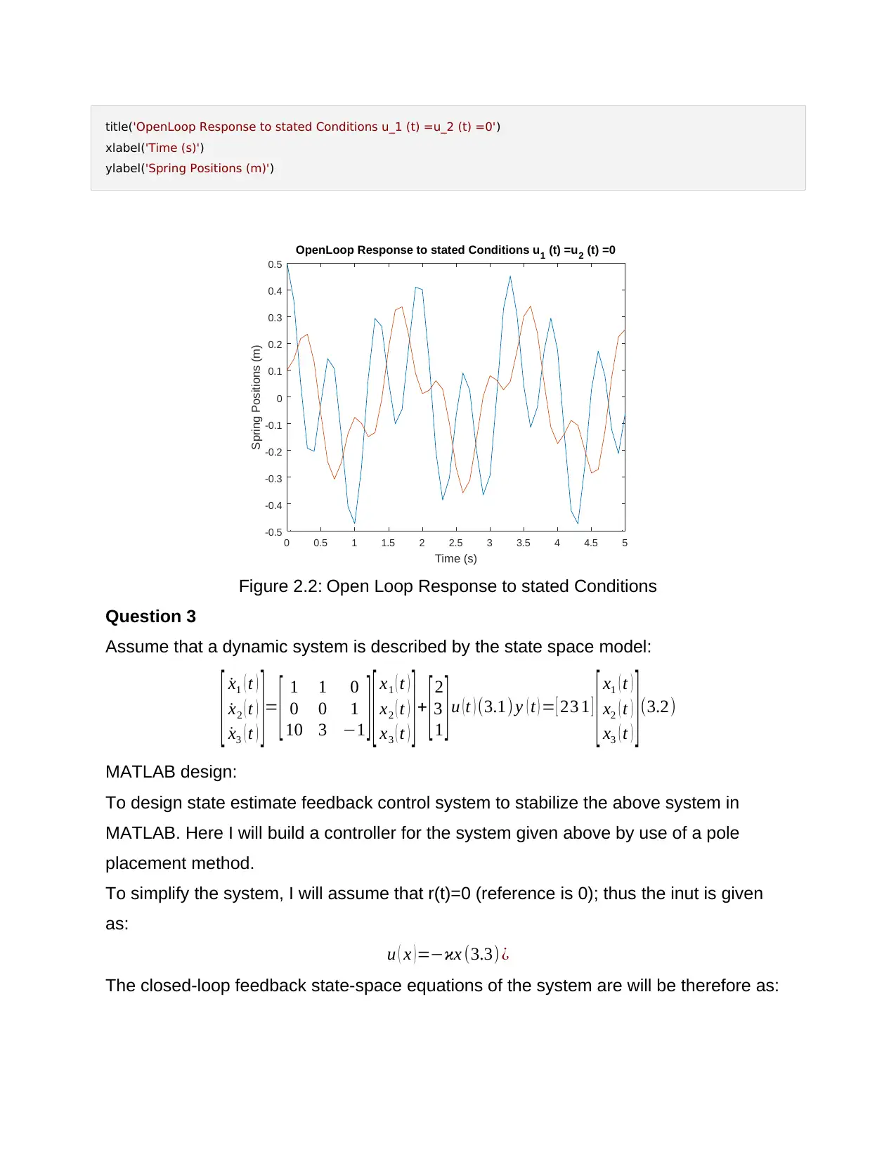
title('OpenLoop Response to stated Conditions u_1 (t) =u_2 (t) =0')
xlabel('Time (s)')
ylabel('Spring Positions (m)')
0 0.5 1 1.5 2 2.5 3 3.5 4 4.5 5
Time (s)
-0.5
-0.4
-0.3
-0.2
-0.1
0
0.1
0.2
0.3
0.4
0.5
Spring Positions (m)
OpenLoop Response to stated Conditions u1 (t) =u2 (t) =0
Figure 2.2: Open Loop Response to stated Conditions
Question 3
Assume that a dynamic system is described by the state space model:
[ ˙x1 ( t )
˙x2 ( t )
˙x3 ( t ) ]= [ 1 1 0
0 0 1
10 3 −1 ] [ x1 ( t )
x2 ( t )
x3 ( t ) ]+ [2
3
1 ]u (t ) (3.1) y ( t ) = [ 23 1 ] [ x1 ( t )
x2 ( t )
x3 ( t ) ](3.2)
MATLAB design:
To design state estimate feedback control system to stabilize the above system in
MATLAB. Here I will build a controller for the system given above by use of a pole
placement method.
To simplify the system, I will assume that r(t)=0 (reference is 0); thus the inut is given
as:
u ( x ) =−ϰx (3.3) ¿
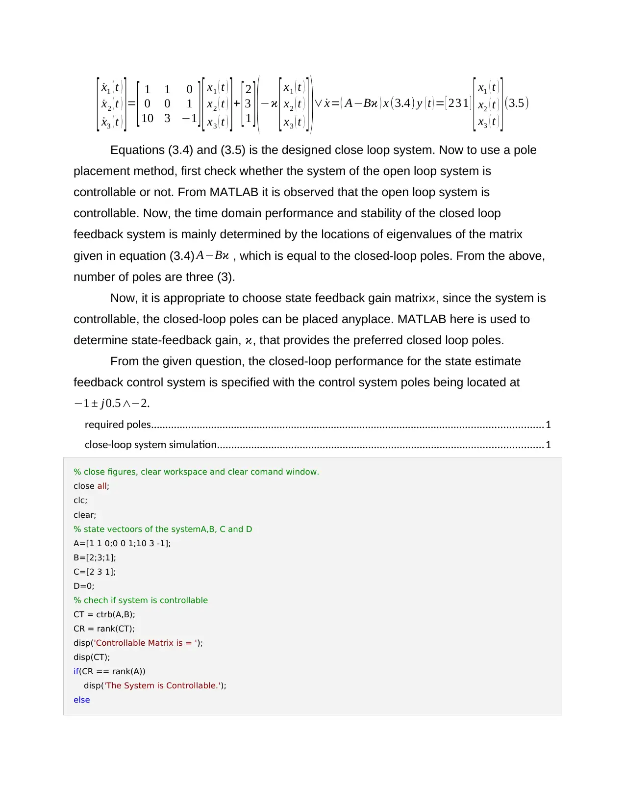
The closed-loop feedback state-space equations of the system are will be therefore as:

[ ˙x1 ( t )
˙x2 ( t )
˙x3 ( t ) ]= [ 1 1 0
0 0 1
10 3 −1 ] [ x1 ( t )
x2 ( t )
x3 ( t ) ]+ [2
3
1 ] (−ϰ
[ x1 ( t )
x2 ( t )
x3 ( t ) ] )∨ ˙x= ( A−Bϰ ) x (3.4) y ( t ) = [ 23 1 ] [ x1 ( t )
x2 ( t )
x3 ( t ) ] (3.5)
Equations (3.4) and (3.5) is the designed close loop system. Now to use a pole
placement method, first check whether the system of the open loop system is
controllable or not. From MATLAB it is observed that the open loop system is
controllable. Now, the time domain performance and stability of the closed loop
feedback system is mainly determined by the locations of eigenvalues of the matrix
given in equation (3.4) A−Bϰ , which is equal to the closed-loop poles. From the above,
number of poles are three (3).
Now, it is appropriate to choose state feedback gain matrixϰ, since the system is
controllable, the closed-loop poles can be placed anyplace. MATLAB here is used to
determine state-feedback gain, ϰ, that provides the preferred closed loop poles.
From the given question, the closed-loop performance for the state estimate
feedback control system is specified with the control system poles being located at
−1 ± j0.5∧−2.
required poles.........................................................................................................................................1
close-loop system simulation..................................................................................................................1
% close figures, clear workspace and clear comand window.
close all;
clc;
clear;
% state vectoors of the systemA,B, C and D
A=[1 1 0;0 0 1;10 3 -1];
B=[2;3;1];
C=[2 3 1];
D=0;
% chech if system is controllable
CT = ctrb(A,B);
CR = rank(CT);
disp('Controllable Matrix is = ');
disp(CT);
if(CR == rank(A))
disp('The System is Controllable.');
else

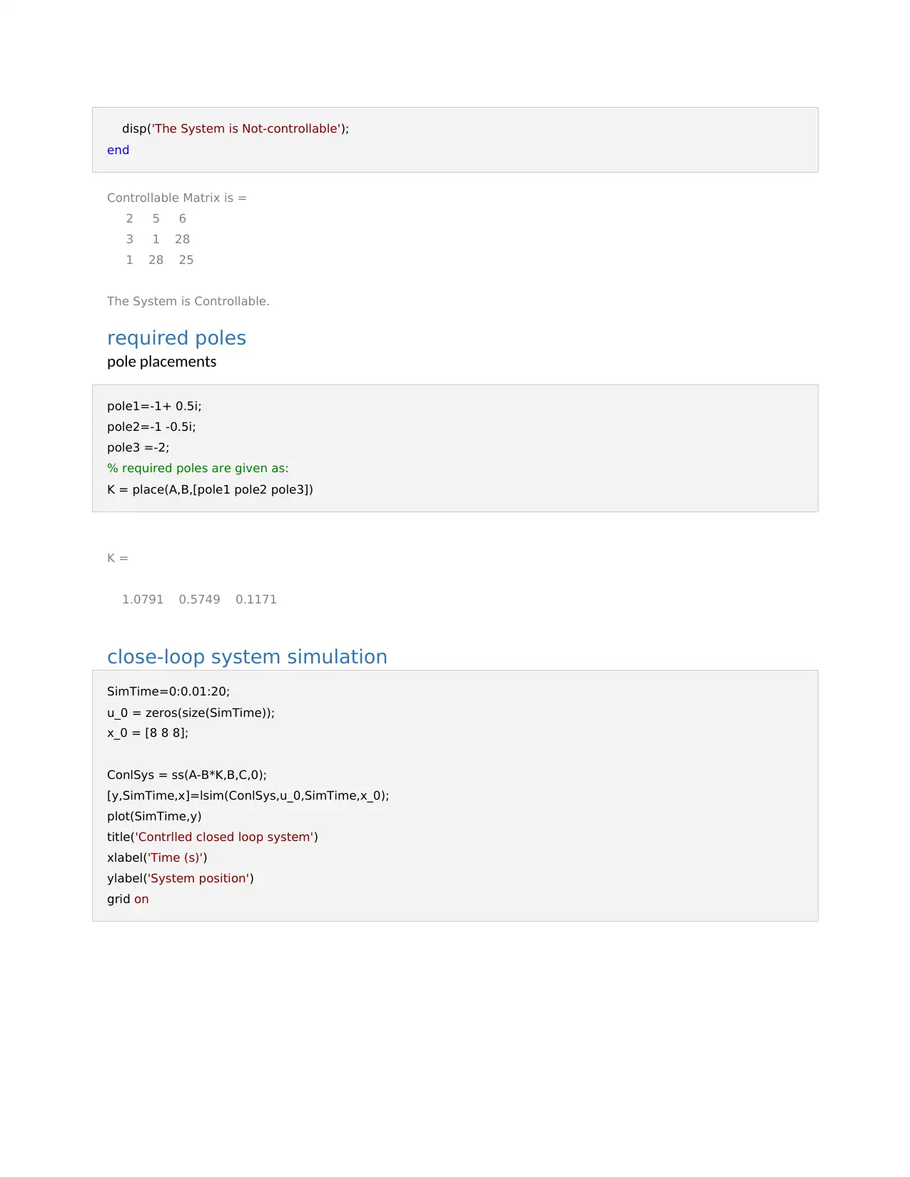
disp('The System is Not-controllable');
end
Controllable Matrix is =
2 5 6
3 1 28
1 28 25
The System is Controllable.
required poles
pole placements
pole1=-1+ 0.5i;
pole2=-1 -0.5i;
pole3 =-2;
% required poles are given as:
K = place(A,B,[pole1 pole2 pole3])
K =
1.0791 0.5749 0.1171
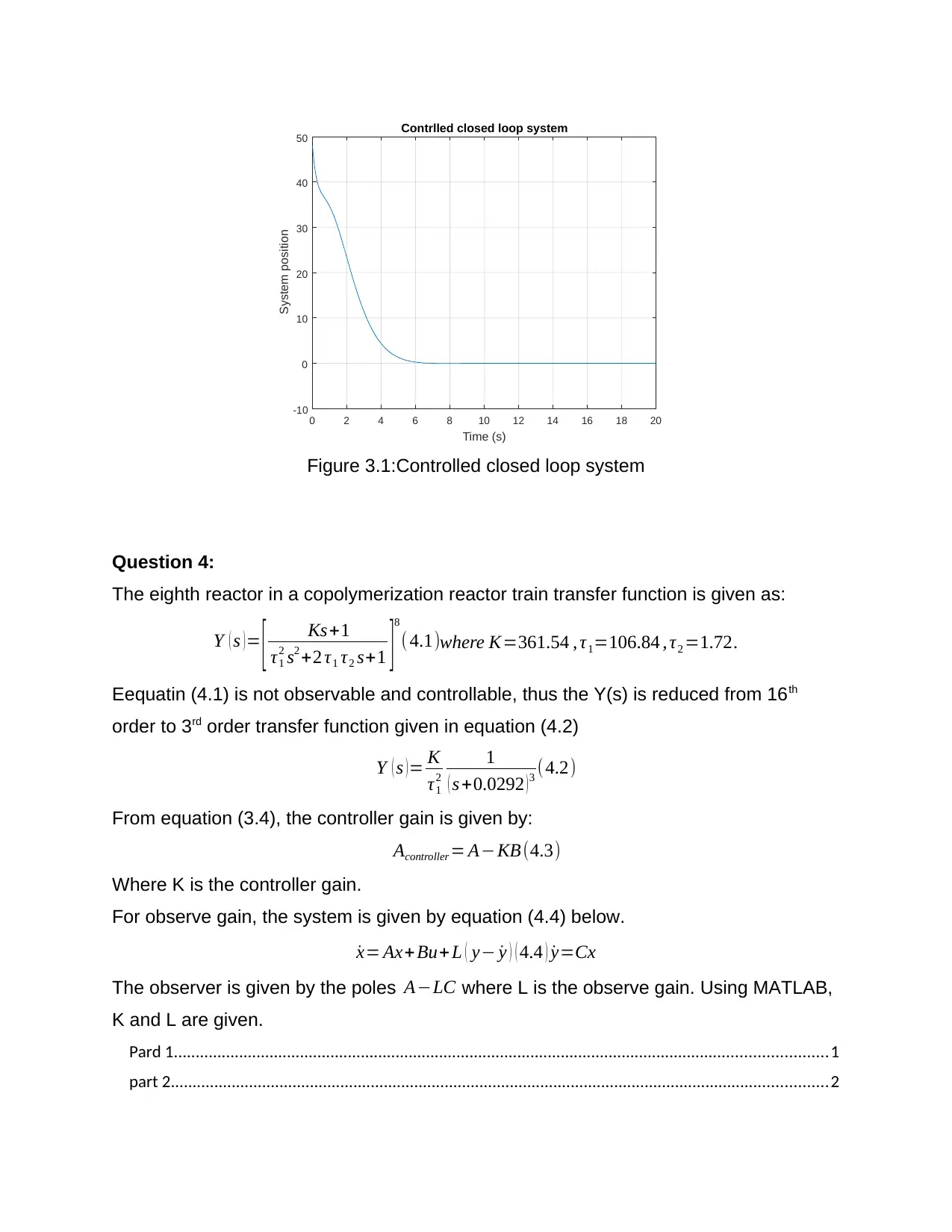
close-loop system simulation
SimTime=0:0.01:20;
u_0 = zeros(size(SimTime));
x_0 = [8 8 8];
ConlSys = ss(A-B*K,B,C,0);
[y,SimTime,x]=lsim(ConlSys,u_0,SimTime,x_0);
plot(SimTime,y)
title('Contrlled closed loop system')
xlabel('Time (s)')
ylabel('System position')
grid on

0 2 4 6 8 10 12 14 16 18 20
Time (s)
-10
0
10
20
30
40
50
System position
Contrlled closed loop system
Figure 3.1:Controlled closed loop system
Question 4:
The eighth reactor in a copolymerization reactor train transfer function is given as:
Y ( s ) = [ Ks+1
τ1
2 s2 +2 τ1 τ2 s+1 ]
8
( 4.1)where K=361.54 , τ1=106.84 , τ2 =1.72.
Eequatin (4.1) is not observable and controllable, thus the Y(s) is reduced from 16th
order to 3rd order transfer function given in equation (4.2)
Y ( s )= K
τ1
2
1
( s +0.0292 )3 (4.2)
From equation (3.4), the controller gain is given by:
Acontroller = A−KB (4.3)
Where K is the controller gain.
For observe gain, the system is given by equation (4.4) below.
˙x= Ax+Bu+ L ( y− ˙y ) ( 4.4 ) ˙y=Cx
The observer is given by the poles A−LC where L is the observe gain. Using MATLAB,
K and L are given.
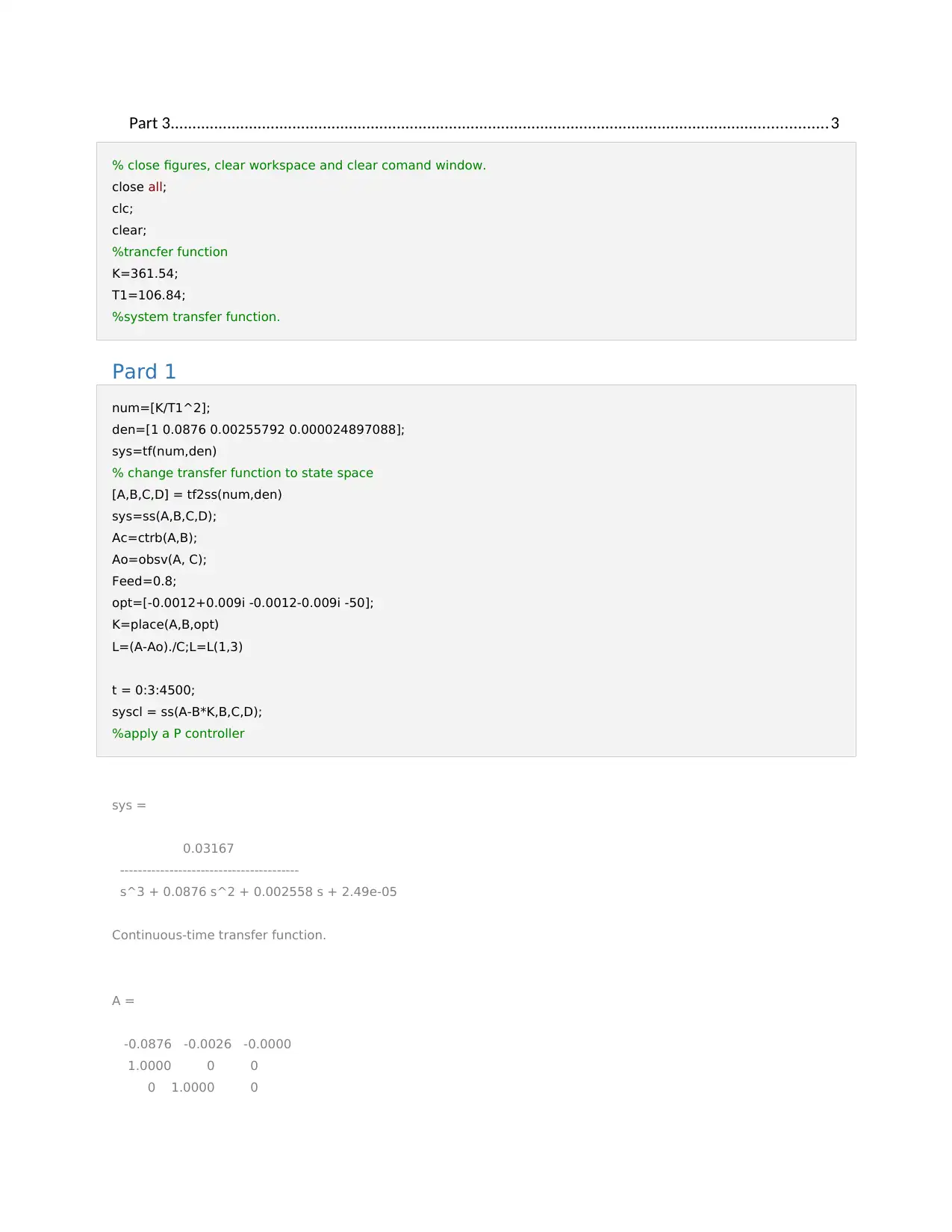
Pard 1......................................................................................................................................................1
part 2.......................................................................................................................................................2

Part 3.......................................................................................................................................................3
% close figures, clear workspace and clear comand window.
close all;
clc;
clear;
%trancfer function
K=361.54;
T1=106.84;
%system transfer function.
Pard 1
num=[K/T1^2];
den=[1 0.0876 0.00255792 0.000024897088];
sys=tf(num,den)
% change transfer function to state space
[A,B,C,D] = tf2ss(num,den)
sys=ss(A,B,C,D);
Ac=ctrb(A,B);
Ao=obsv(A, C);
Feed=0.8;
opt=[-0.0012+0.009i -0.0012-0.009i -50];
K=place(A,B,opt)
L=(A-Ao)./C;L=L(1,3)
t = 0:3:4500;
syscl = ss(A-B*K,B,C,D);
%apply a P controller
sys =
0.03167
----------------------------------------
s^3 + 0.0876 s^2 + 0.002558 s + 2.49e-05
Continuous-time transfer function.
A =
-0.0876 -0.0026 -0.0000
1.0000 0 0
0 1.0000 0

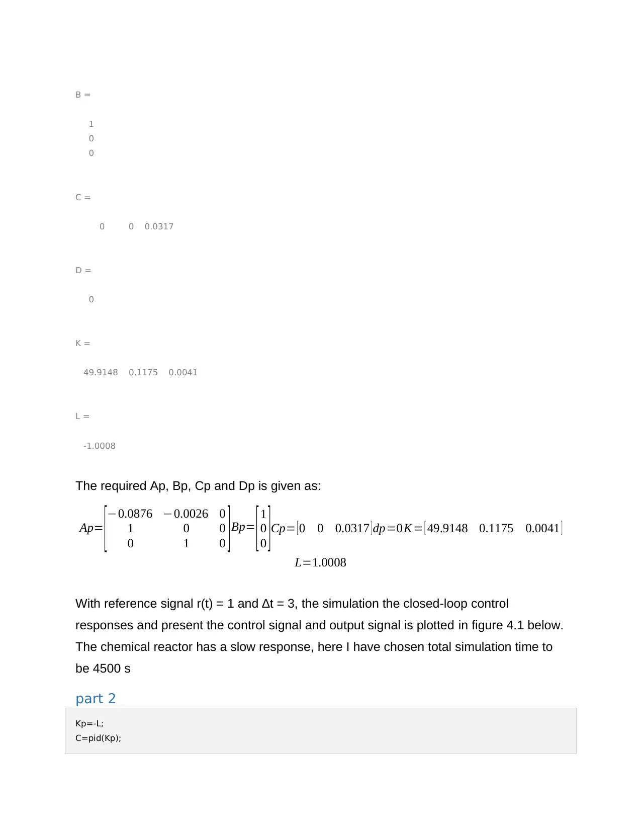
B =
1
0
0
C =
0 0 0.0317
D =
0
K =
49.9148 0.1175 0.0041
L =
-1.0008
The required Ap, Bp, Cp and Dp is given as:
Ap= [−0.0876 −0.0026 0
1 0 0
0 1 0 ] Bp= [ 1
0
0 ]Cp= [ 0 0 0.0317 ]dp=0 K= [ 49.9148 0.1175 0.0041 ]
L=1.0008
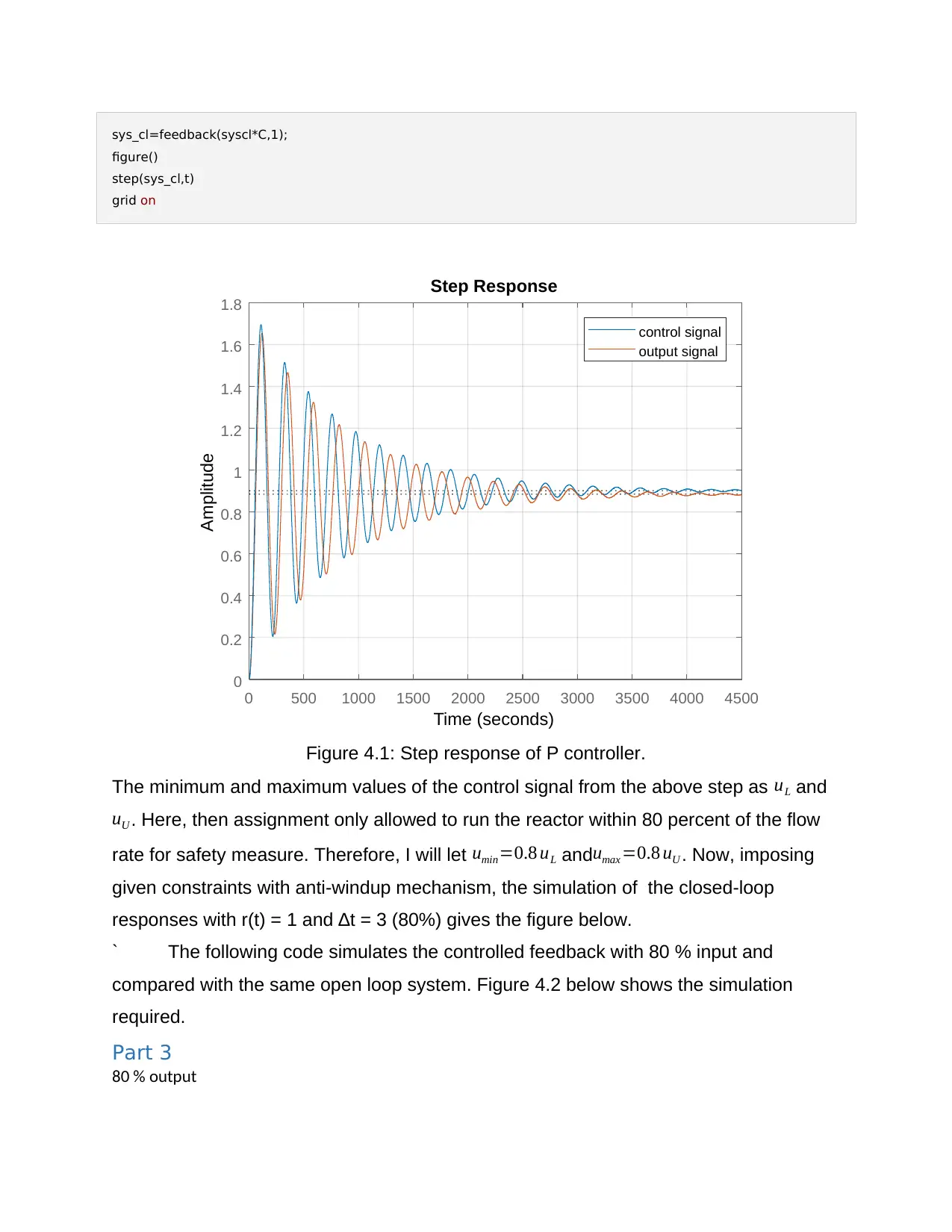
With reference signal r(t) = 1 and ∆t = 3, the simulation the closed-loop control
responses and present the control signal and output signal is plotted in figure 4.1 below.
The chemical reactor has a slow response, here I have chosen total simulation time to
be 4500 s
part 2
Kp=-L;
C=pid(Kp);

sys_cl=feedback(syscl*C,1);
figure()
step(sys_cl,t)
grid on
0 500 1000 1500 2000 2500 3000 3500 4000 4500
0
0.2
0.4
0.6
0.8
1
1.2
1.4
1.6
1.8
control signal
output signal
Step Response
Time (seconds)
Amplitude
Figure 4.1: Step response of P controller.
The minimum and maximum values of the control signal from the above step as uL and
uU . Here, then assignment only allowed to run the reactor within 80 percent of the flow
rate for safety measure. Therefore, I will let umin=0.8 uL andumax =0.8 uU . Now, imposing
given constraints with anti-windup mechanism, the simulation of the closed-loop
responses with r(t) = 1 and ∆t = 3 (80%) gives the figure below.
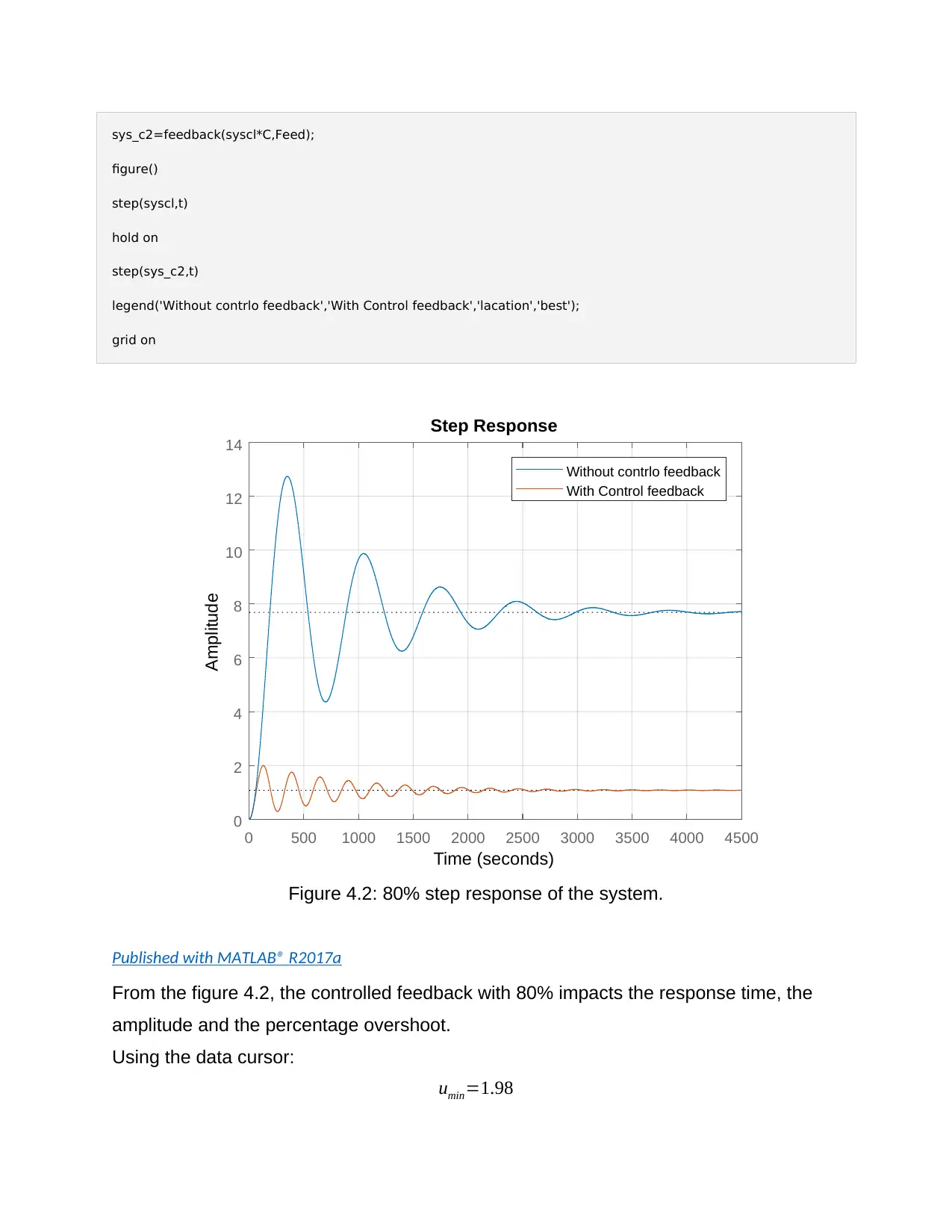
` The following code simulates the controlled feedback with 80 % input and
compared with the same open loop system. Figure 4.2 below shows the simulation
required.
Part 3
80 % output

sys_c2=feedback(syscl*C,Feed);
figure()
step(syscl,t)
hold on
step(sys_c2,t)
legend('Without contrlo feedback','With Control feedback','lacation','best');
grid on
0 500 1000 1500 2000 2500 3000 3500 4000 4500
0
2
4
6
8
10
12
14
Without contrlo feedback
With Control feedback
Step Response
Time (seconds)
Amplitude
Figure 4.2: 80% step response of the system.
Published with MATLAB® R2017a
From the figure 4.2, the controlled feedback with 80% impacts the response time, the
amplitude and the percentage overshoot.
Using the data cursor:
umin=1.98

umax=0.287