Study on the Vehicle Routing Problem
Added on 2020-05-04
12 Pages4924 Words51 Views
VEHICLE ROUTINGINTRODUCTIONThe vehicle routing problem with capacity constraints is one of the common subject of study.The main is to design the least cost routes for fleet of vehicles from one point to the set points.Vehicles belong to a fleet located to the central depot and have a capacity .The cost of each customer’s travel depends on the distance travelling .The algorithm in use here is the based on thr heuristic approach and is based on Ropke pisinger in terms of ALNS ABSTRACTVRP consists of the problems in which a set of routes for a fleet of vehicles based at one or several depots must be established for a number of geographically dispersed cities or customers .The aim here is to find the set of routes at a minimal cost basically finding the shortest path,minimizing the number ofvehicles and others.NOTE:CVRP is same as VRPThe mathematical formula would be;A capacity of each vehicleV maximum number of vehiclesFij thye flow of cores from node i to jZ total transportation costDi demand at node iCij Distance between node I and jXi,j{1,0 if vehicle moves from node I to j 0 otherwiseN number of nodesThe model constraints are:\mathop \sum \limits_{l = 2, a\ne l}^{N} x_{la} + x_{1a} = 1\quad \quad \for all a(2)\mathop \sum \limits_{l = 2, a \ne l}^{N} x_{al} + x_{a1} = 1\quad \quad \for all a(3)
\mathop \sum \limits_{a = 2}^{N} x_{1a} \le V(4)\mathop \sum \limits_{j = 1, j \ne i}^{N} x_{ij} = \mathop \sum \limits_{j = 1, j \ne i}^{N} x_{ji} \quad \quad \for all i(5)x_{aa} = 0\quad \quad \forall a(6)x_{la} + x_{al} = 1\quad \quad \for all a, \, l_{a \ne 1}(7)\mathop \sum \limits_{j = 1,j \ne i}^{N} F_{ij} = \mathop \sum \limits_{j = 1,j \ne i}^{N} F_{ji} + d_{i} \quad \quad \for all i_{i > 1}(8)d_{i} .x_{ij} \le F_{ij} \quad \quad \for all i,j_{i \ne j}(9)F_{ij} \le \left( {A - d_{j} } \right).x_{ij} \quad \quad \for all i,j_{i \ne j}(10)The objective function (1) of the model is to minimize the total traveled distance. The constraints (2) and(3) state that there is exactly one departure from node i. The constraint (4) provides not to exceed the total number of vehicles. Constraint (5) provides balance between incoming and outgoing arcs at a givennode. Constraint (6) eliminates flow from node i to node i. Constraint (7) is trivial sub-tour elimination constraint. Constraints (8), (9) and (10) provide balance between total inflow and outflow at node.This mathematical model can be used for only small-scale CVRP because it is quite difficult to achieve an optimal solution with traditional optimization methods due to the high computational complexity for large-scale problems. For this reason, we constructed a novel heuristic algorithm for CVRP in this study.algorithm for CVRPIn this section, our proposed algorithm is explained. We used following notation in the algorithm. The points to visit are denoted by a set of S which has number of p elements as S = \left\{ {1, \ldots , \, p} \right\}. All the points are also denoted analytically by an arc set of P as P = \left\{ {\left( {x_{i} , \, y_{i} } \right):\,\,i\,\, \in \,\,S} \right\}. \Delta_{ij} = \left( {\left( {x_{i} - x_{j} } \right)^{2} + \left( {y_{i} - y_{j} } \right)^{2} } \right)^{0.5} is the distance matrix which states the distance between the elements of S set. A solution is the sets R of k routes and also vehicles, Rk⊆S and k are less than and equal to the number
of free vehicle t. All the points to visit have a demand di and the capacity of free vehicles meeting the total demand is assumed as \varSigma d_{i} \le tC. We determined the objective function asF = \var Sigma_{a = 1}^{t} \var Sigma_{i = 1}^{p} \var Sigma_{j = 1}^{p} \pi_{ija} \Delta_{ij} \;{\text{for all}}\,\,i, \, j\, \in S, \, i \ne j{\text{ and }}a \le t,where\pi_{ija} = \left\{ {\begin{array}{*{20}l} 1 \hfill & {{\text{from}}\,\,i\,\,{\text{to}}\,\,j\,\,{\text{by}}\,\,{\text{vehicle}}\,\,a} \hfill \\ 0 \hfill & {\text{otherwise}} \hfill \\ \end{array} } \right..The capacity constraints must be kept down while searching for a solution. Therefore, we determined a function to control the feasibility of the candidate solution as \sum\nolimits_{a= 1}^{t} {\pi_{ija} d_{j} \le C }\;{\text{for all}}\;i, j \in S\;{\text{and}}\;i \ne j .One of our motivations is that the quality of initial solution affected the performance of the algorithm. Hence, we prefer to start the solution by these steps:Step 1: Start from a random i point and determine the πijk as 1 considering the minimum value of Δij, where the S=S* and Rk=Rk*.Step 2: Calculate the \bar{C}_{a} = C_{a} + d_{j} and S* = S\backslash \left\{ j \right\} and R_{a} * = R_{a} \, \cup \,\left\{ j \right\}.Step 3: Repeat steps 1 and 2 up to \bar{C}_{a} \ge C. When this is met, increase the value of a as 1.Step 4: Run the all previous steps until S* \in ∅. At last all of Rk* state us the solution.After determining the initial solution, new solutions are determined by ALNS. In this study, we constructed a relocation procedure to search neighborhoods. The steps of the procedure consist of these steps:Stage 1: Select one of each point i from each routes Rk* by roulette wheel principle using Eq.p_{a} = \frac{{\sum\nolimits_{i = 1}^{p} {\sum\limits_{j = 1}^{p} {\pi_{ija} \Delta_{ij} } } }}{{\sum\nolimits_{a = 1}^{t} {\sum\limits_{i = 1}^{p} {\sum\limits_{j = 1}^{p} {\pi_{ija} \Delta_{ij} } } } }}.(11)Stage 2: Determine the second closest points to each selected points according to the Δij matrix.Stage 3: Start from the R1 and relocate the selected point with its second closest point. If the selected point and its second point are in the same route, do not relocate them. So we can prevent to enhance the solution space too much.Stage 3 : While relocating, \bar{C}_{a} = C_{a} + d_{j} should be revised and route capacity should be ′controlled.Stage 4: Stages 2 and 3 are repeated for all the points which were selected in Stage 1.
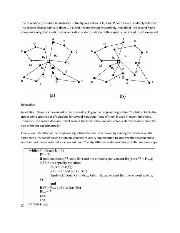
The relocation procedure is illustrated in the figures below D, H, J and P points were randomly selected. The second closest points to them E, I, H and A were chosen respectively. Part (b) of the second figure shows us a neighbor solution after relocation under condition of the capacity constraint in not exceeded.RelocationIn addition, there is a movement list to prevent cycling in the proposed algorithm. This list prohibits the use of some specific set of solutions for several iterations if one of them is used in recent iterations. Therefore, the search does not travel around the local optimum points. We preferred to determine the size of the list experimentally.Finally, each iteration of the proposed algorithm that can be achieved by serving two vertices on the same route instead of leaving them on separate routes is implemented to improve the solution and a non-tabu solution is selected as a new solution. The algorithm after determining an initial solution steps w
End of preview
Want to access all the pages? Upload your documents or become a member.