Sum Function Sales (Part A)
VerifiedAdded on 2023/04/23
|9
|2188
|114
AI Summary
Contribute Materials
Your contribution can guide someone’s learning journey. Share your
documents today.
Accounts
PART A
Answer 1
The three excel functions that I have used and found them useful has been described here-in-
below:
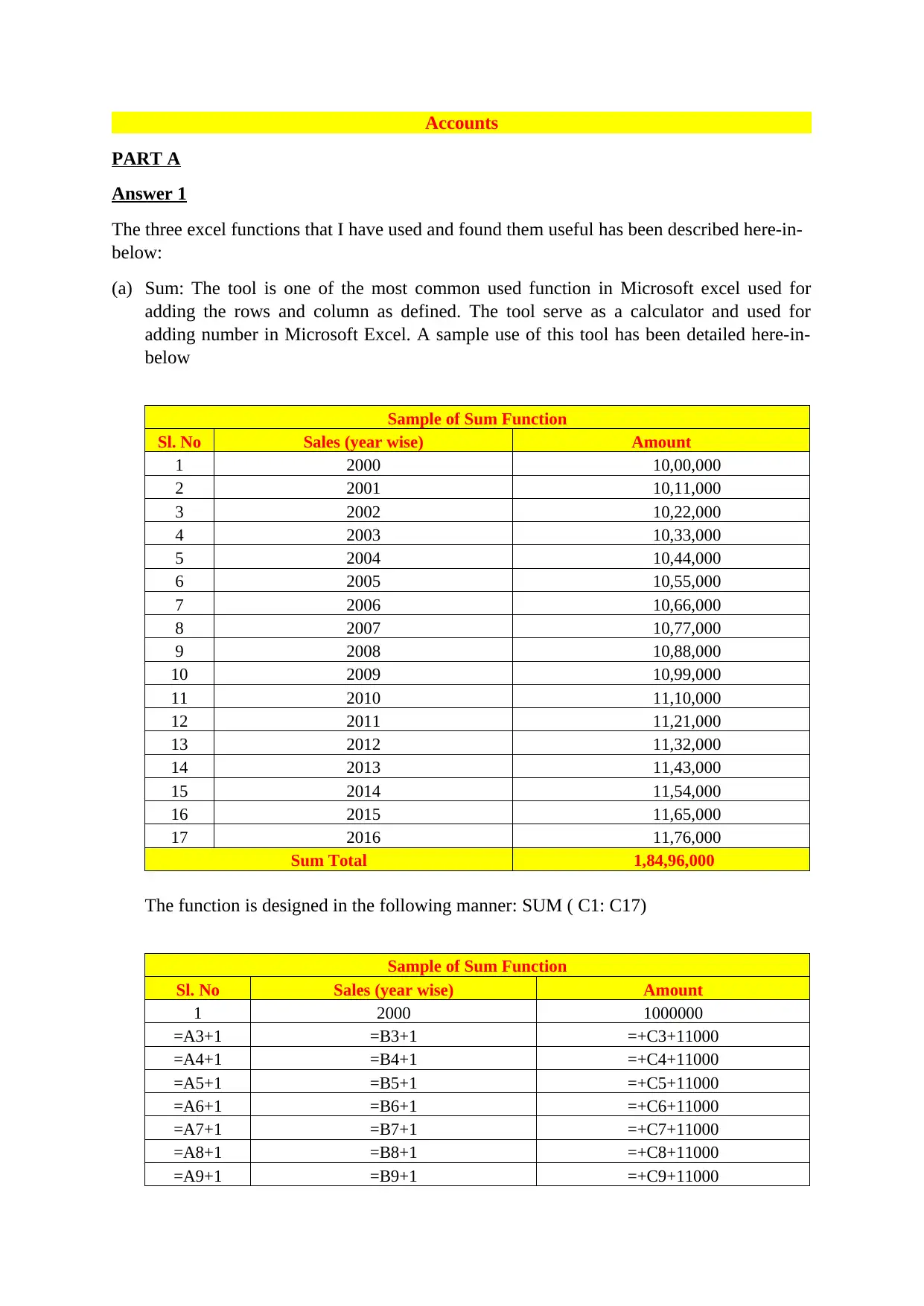
(a) Sum: The tool is one of the most common used function in Microsoft excel used for
adding the rows and column as defined. The tool serve as a calculator and used for
adding number in Microsoft Excel. A sample use of this tool has been detailed here-in-
below
Sample of Sum Function
Sl. No Sales (year wise) Amount
1 2000 10,00,000
2 2001 10,11,000
3 2002 10,22,000
4 2003 10,33,000
5 2004 10,44,000
6 2005 10,55,000
7 2006 10,66,000
8 2007 10,77,000
9 2008 10,88,000
10 2009 10,99,000
11 2010 11,10,000
12 2011 11,21,000
13 2012 11,32,000
14 2013 11,43,000
15 2014 11,54,000
16 2015 11,65,000
17 2016 11,76,000
Sum Total 1,84,96,000
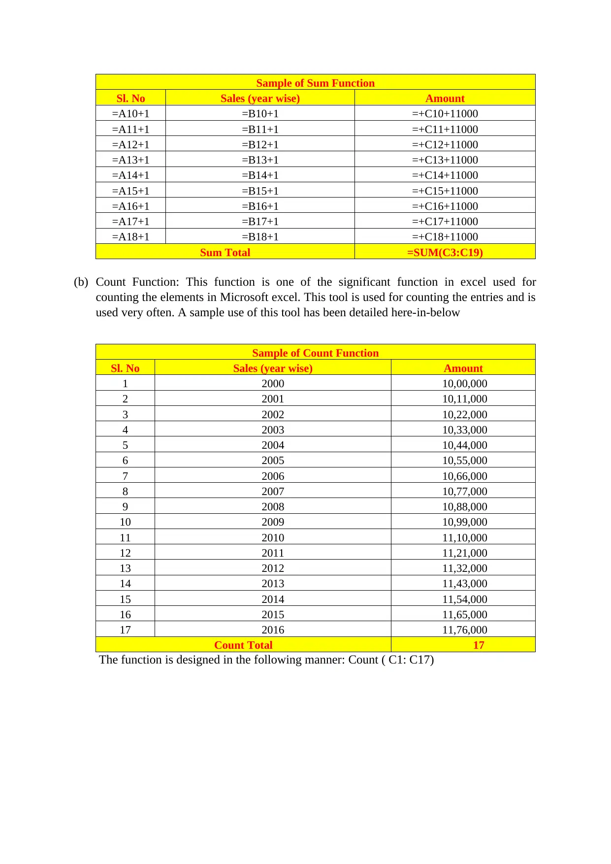
The function is designed in the following manner: SUM ( C1: C17)
Sample of Sum Function
Sl. No Sales (year wise) Amount
1 2000 1000000
=A3+1 =B3+1 =+C3+11000
=A4+1 =B4+1 =+C4+11000
=A5+1 =B5+1 =+C5+11000
=A6+1 =B6+1 =+C6+11000
=A7+1 =B7+1 =+C7+11000
=A8+1 =B8+1 =+C8+11000
=A9+1 =B9+1 =+C9+11000
Secure Best Marks with AI Grader
Need help grading? Try our AI Grader for instant feedback on your assignments.
Sample of Sum Function
Sl. No Sales (year wise) Amount
=A10+1 =B10+1 =+C10+11000
=A11+1 =B11+1 =+C11+11000
=A12+1 =B12+1 =+C12+11000
=A13+1 =B13+1 =+C13+11000
=A14+1 =B14+1 =+C14+11000
=A15+1 =B15+1 =+C15+11000
=A16+1 =B16+1 =+C16+11000
=A17+1 =B17+1 =+C17+11000
=A18+1 =B18+1 =+C18+11000
Sum Total =SUM(C3:C19)
(b) Count Function: This function is one of the significant function in excel used for
counting the elements in Microsoft excel. This tool is used for counting the entries and is
used very often. A sample use of this tool has been detailed here-in-below
Sample of Count Function
Sl. No Sales (year wise) Amount
1 2000 10,00,000
2 2001 10,11,000
3 2002 10,22,000
4 2003 10,33,000
5 2004 10,44,000
6 2005 10,55,000
7 2006 10,66,000
8 2007 10,77,000
9 2008 10,88,000
10 2009 10,99,000
11 2010 11,10,000
12 2011 11,21,000
13 2012 11,32,000
14 2013 11,43,000
15 2014 11,54,000
16 2015 11,65,000
17 2016 11,76,000
Count Total 17
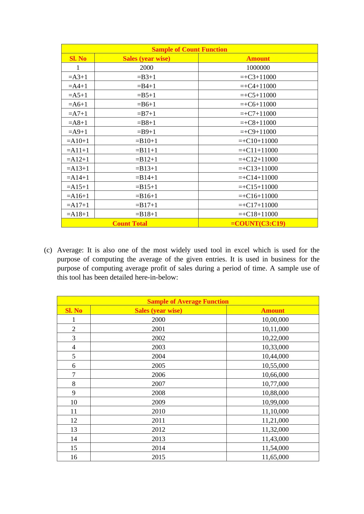
The function is designed in the following manner: Count ( C1: C17)
Sl. No Sales (year wise) Amount
=A10+1 =B10+1 =+C10+11000
=A11+1 =B11+1 =+C11+11000
=A12+1 =B12+1 =+C12+11000
=A13+1 =B13+1 =+C13+11000
=A14+1 =B14+1 =+C14+11000
=A15+1 =B15+1 =+C15+11000
=A16+1 =B16+1 =+C16+11000
=A17+1 =B17+1 =+C17+11000
=A18+1 =B18+1 =+C18+11000
Sum Total =SUM(C3:C19)
(b) Count Function: This function is one of the significant function in excel used for
counting the elements in Microsoft excel. This tool is used for counting the entries and is
used very often. A sample use of this tool has been detailed here-in-below
Sample of Count Function
Sl. No Sales (year wise) Amount
1 2000 10,00,000
2 2001 10,11,000
3 2002 10,22,000
4 2003 10,33,000
5 2004 10,44,000
6 2005 10,55,000
7 2006 10,66,000
8 2007 10,77,000
9 2008 10,88,000
10 2009 10,99,000
11 2010 11,10,000
12 2011 11,21,000
13 2012 11,32,000
14 2013 11,43,000
15 2014 11,54,000
16 2015 11,65,000
17 2016 11,76,000
Count Total 17
The function is designed in the following manner: Count ( C1: C17)
Sample of Count Function
Sl. No Sales (year wise) Amount
1 2000 1000000
=A3+1 =B3+1 =+C3+11000
=A4+1 =B4+1 =+C4+11000
=A5+1 =B5+1 =+C5+11000
=A6+1 =B6+1 =+C6+11000
=A7+1 =B7+1 =+C7+11000
=A8+1 =B8+1 =+C8+11000
=A9+1 =B9+1 =+C9+11000
=A10+1 =B10+1 =+C10+11000
=A11+1 =B11+1 =+C11+11000
=A12+1 =B12+1 =+C12+11000
=A13+1 =B13+1 =+C13+11000
=A14+1 =B14+1 =+C14+11000
=A15+1 =B15+1 =+C15+11000
=A16+1 =B16+1 =+C16+11000
=A17+1 =B17+1 =+C17+11000
=A18+1 =B18+1 =+C18+11000
Count Total =COUNT(C3:C19)
(c) Average: It is also one of the most widely used tool in excel which is used for the
purpose of computing the average of the given entries. It is used in business for the
purpose of computing average profit of sales during a period of time. A sample use of
this tool has been detailed here-in-below:
Sample of Average Function
Sl. No Sales (year wise) Amount
1 2000 10,00,000
2 2001 10,11,000
3 2002 10,22,000
4 2003 10,33,000
5 2004 10,44,000
6 2005 10,55,000
7 2006 10,66,000
8 2007 10,77,000
9 2008 10,88,000
10 2009 10,99,000
11 2010 11,10,000
12 2011 11,21,000
13 2012 11,32,000
14 2013 11,43,000
15 2014 11,54,000
16 2015 11,65,000
Sl. No Sales (year wise) Amount
1 2000 1000000
=A3+1 =B3+1 =+C3+11000
=A4+1 =B4+1 =+C4+11000
=A5+1 =B5+1 =+C5+11000
=A6+1 =B6+1 =+C6+11000
=A7+1 =B7+1 =+C7+11000
=A8+1 =B8+1 =+C8+11000
=A9+1 =B9+1 =+C9+11000
=A10+1 =B10+1 =+C10+11000
=A11+1 =B11+1 =+C11+11000
=A12+1 =B12+1 =+C12+11000
=A13+1 =B13+1 =+C13+11000
=A14+1 =B14+1 =+C14+11000
=A15+1 =B15+1 =+C15+11000
=A16+1 =B16+1 =+C16+11000
=A17+1 =B17+1 =+C17+11000
=A18+1 =B18+1 =+C18+11000
Count Total =COUNT(C3:C19)
(c) Average: It is also one of the most widely used tool in excel which is used for the
purpose of computing the average of the given entries. It is used in business for the
purpose of computing average profit of sales during a period of time. A sample use of
this tool has been detailed here-in-below:
Sample of Average Function
Sl. No Sales (year wise) Amount
1 2000 10,00,000
2 2001 10,11,000
3 2002 10,22,000
4 2003 10,33,000
5 2004 10,44,000
6 2005 10,55,000
7 2006 10,66,000
8 2007 10,77,000
9 2008 10,88,000
10 2009 10,99,000
11 2010 11,10,000
12 2011 11,21,000
13 2012 11,32,000
14 2013 11,43,000
15 2014 11,54,000
16 2015 11,65,000
Sample of Average Function
Sl. No Sales (year wise) Amount
17 2016 11,76,000
Average 10,88,000
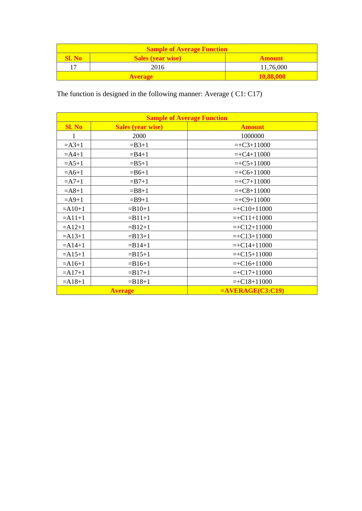
The function is designed in the following manner: Average ( C1: C17)
Sample of Average Function
Sl. No Sales (year wise) Amount
1 2000 1000000
=A3+1 =B3+1 =+C3+11000
=A4+1 =B4+1 =+C4+11000
=A5+1 =B5+1 =+C5+11000
=A6+1 =B6+1 =+C6+11000
=A7+1 =B7+1 =+C7+11000
=A8+1 =B8+1 =+C8+11000
=A9+1 =B9+1 =+C9+11000
=A10+1 =B10+1 =+C10+11000
=A11+1 =B11+1 =+C11+11000
=A12+1 =B12+1 =+C12+11000
=A13+1 =B13+1 =+C13+11000
=A14+1 =B14+1 =+C14+11000
=A15+1 =B15+1 =+C15+11000
=A16+1 =B16+1 =+C16+11000
=A17+1 =B17+1 =+C17+11000
=A18+1 =B18+1 =+C18+11000
Average =AVERAGE(C3:C19)
Sl. No Sales (year wise) Amount
17 2016 11,76,000
Average 10,88,000
The function is designed in the following manner: Average ( C1: C17)
Sample of Average Function
Sl. No Sales (year wise) Amount
1 2000 1000000
=A3+1 =B3+1 =+C3+11000
=A4+1 =B4+1 =+C4+11000
=A5+1 =B5+1 =+C5+11000
=A6+1 =B6+1 =+C6+11000
=A7+1 =B7+1 =+C7+11000
=A8+1 =B8+1 =+C8+11000
=A9+1 =B9+1 =+C9+11000
=A10+1 =B10+1 =+C10+11000
=A11+1 =B11+1 =+C11+11000
=A12+1 =B12+1 =+C12+11000
=A13+1 =B13+1 =+C13+11000
=A14+1 =B14+1 =+C14+11000
=A15+1 =B15+1 =+C15+11000
=A16+1 =B16+1 =+C16+11000
=A17+1 =B17+1 =+C17+11000
=A18+1 =B18+1 =+C18+11000
Average =AVERAGE(C3:C19)
Secure Best Marks with AI Grader
Need help grading? Try our AI Grader for instant feedback on your assignments.
Answer 2
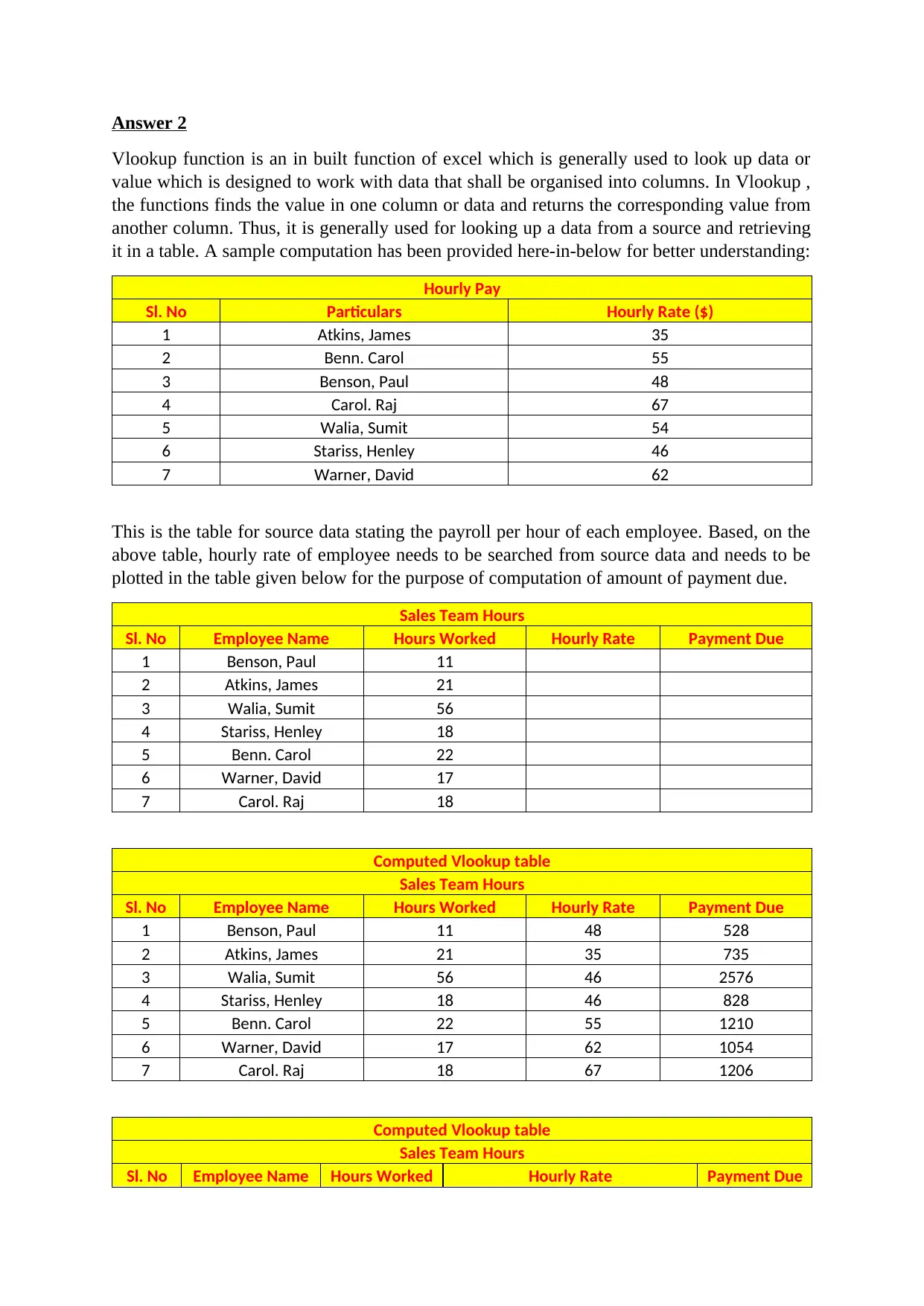
Vlookup function is an in built function of excel which is generally used to look up data or
value which is designed to work with data that shall be organised into columns. In Vlookup ,
the functions finds the value in one column or data and returns the corresponding value from
another column. Thus, it is generally used for looking up a data from a source and retrieving
it in a table. A sample computation has been provided here-in-below for better understanding:
Hourly Pay
Sl. No Particulars Hourly Rate ($)
1 Atkins, James 35
2 Benn. Carol 55
3 Benson, Paul 48
4 Carol. Raj 67
5 Walia, Sumit 54
6 Stariss, Henley 46
7 Warner, David 62
This is the table for source data stating the payroll per hour of each employee. Based, on the
above table, hourly rate of employee needs to be searched from source data and needs to be
plotted in the table given below for the purpose of computation of amount of payment due.
Sales Team Hours
Sl. No Employee Name Hours Worked Hourly Rate Payment Due
1 Benson, Paul 11
2 Atkins, James 21
3 Walia, Sumit 56
4 Stariss, Henley 18
5 Benn. Carol 22
6 Warner, David 17
7 Carol. Raj 18
Computed Vlookup table
Sales Team Hours
Sl. No Employee Name Hours Worked Hourly Rate Payment Due
1 Benson, Paul 11 48 528
2 Atkins, James 21 35 735
3 Walia, Sumit 56 46 2576
4 Stariss, Henley 18 46 828
5 Benn. Carol 22 55 1210
6 Warner, David 17 62 1054
7 Carol. Raj 18 67 1206
Computed Vlookup table
Sales Team Hours
Sl. No Employee Name Hours Worked Hourly Rate Payment Due
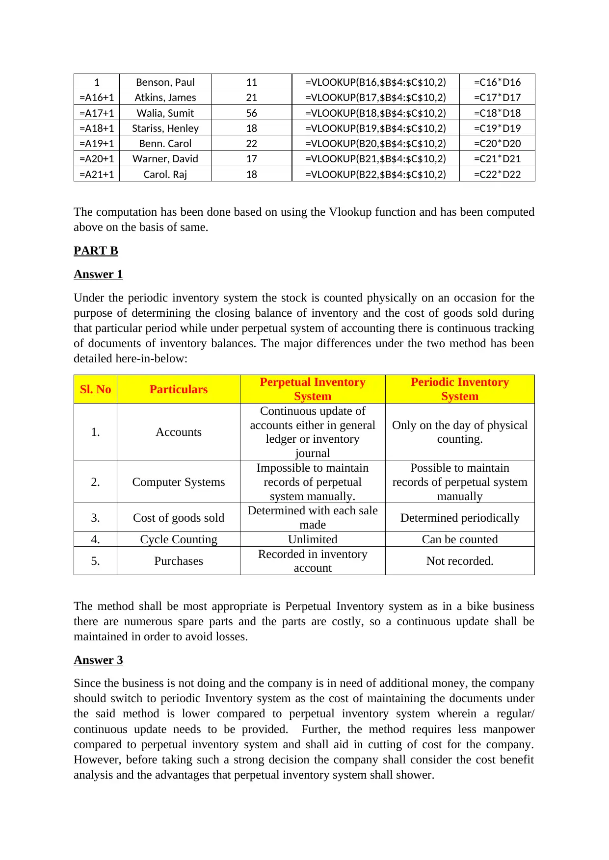
1 Benson, Paul 11 =VLOOKUP(B16,$B$4:$C$10,2) =C16*D16
=A16+1 Atkins, James 21 =VLOOKUP(B17,$B$4:$C$10,2) =C17*D17
=A17+1 Walia, Sumit 56 =VLOOKUP(B18,$B$4:$C$10,2) =C18*D18
=A18+1 Stariss, Henley 18 =VLOOKUP(B19,$B$4:$C$10,2) =C19*D19
=A19+1 Benn. Carol 22 =VLOOKUP(B20,$B$4:$C$10,2) =C20*D20
=A20+1 Warner, David 17 =VLOOKUP(B21,$B$4:$C$10,2) =C21*D21
=A21+1 Carol. Raj 18 =VLOOKUP(B22,$B$4:$C$10,2) =C22*D22
The computation has been done based on using the Vlookup function and has been computed
above on the basis of same.
PART B
Answer 1
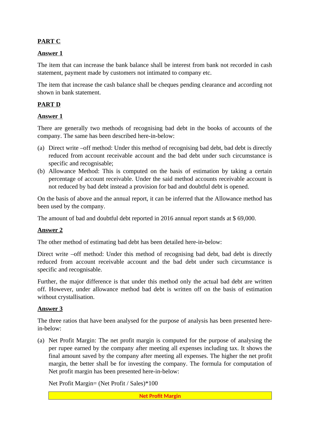
Under the periodic inventory system the stock is counted physically on an occasion for the
purpose of determining the closing balance of inventory and the cost of goods sold during
that particular period while under perpetual system of accounting there is continuous tracking
of documents of inventory balances. The major differences under the two method has been
detailed here-in-below:
Sl. No Particulars Perpetual Inventory
System
Periodic Inventory
System
1. Accounts
Continuous update of
accounts either in general
ledger or inventory
journal
Only on the day of physical
counting.
2. Computer Systems
Impossible to maintain
records of perpetual
system manually.
Possible to maintain
records of perpetual system
manually
3. Cost of goods sold Determined with each sale
made Determined periodically
4. Cycle Counting Unlimited Can be counted
5. Purchases Recorded in inventory
account Not recorded.
The method shall be most appropriate is Perpetual Inventory system as in a bike business
there are numerous spare parts and the parts are costly, so a continuous update shall be
maintained in order to avoid losses.
Answer 3
Since the business is not doing and the company is in need of additional money, the company
should switch to periodic Inventory system as the cost of maintaining the documents under
the said method is lower compared to perpetual inventory system wherein a regular/
continuous update needs to be provided. Further, the method requires less manpower
compared to perpetual inventory system and shall aid in cutting of cost for the company.
However, before taking such a strong decision the company shall consider the cost benefit
analysis and the advantages that perpetual inventory system shall shower.
PART C
Answer 1
The item that can increase the bank balance shall be interest from bank not recorded in cash
statement, payment made by customers not intimated to company etc.
The item that increase the cash balance shall be cheques pending clearance and according not
shown in bank statement.
PART D
Answer 1
There are generally two methods of recognising bad debt in the books of accounts of the
company. The same has been described here-in-below:
(a) Direct write –off method: Under this method of recognising bad debt, bad debt is directly
reduced from account receivable account and the bad debt under such circumstance is
specific and recognisable;
(b) Allowance Method: This is computed on the basis of estimation by taking a certain
percentage of account receivable. Under the said method accounts receivable account is
not reduced by bad debt instead a provision for bad and doubtful debt is opened.
On the basis of above and the annual report, it can be inferred that the Allowance method has
been used by the company.
The amount of bad and doubtful debt reported in 2016 annual report stands at $ 69,000.
Answer 2
The other method of estimating bad debt has been detailed here-in-below:
Direct write –off method: Under this method of recognising bad debt, bad debt is directly
reduced from account receivable account and the bad debt under such circumstance is
specific and recognisable.
Further, the major difference is that under this method only the actual bad debt are written
off. However, under allowance method bad debt is written off on the basis of estimation
without crystallisation.
Answer 3
The three ratios that have been analysed for the purpose of analysis has been presented here-
in-below:
(a) Net Profit Margin: The net profit margin is computed for the purpose of analysing the
per rupee earned by the company after meeting all expenses including tax. It shows the
final amount saved by the company after meeting all expenses. The higher the net profit
margin, the better shall be for investing the company. The formula for computation of
Net profit margin has been presented here-in-below:
Net Profit Margin= (Net Profit / Sales)*100
Net Profit Margin
Answer 1
The item that can increase the bank balance shall be interest from bank not recorded in cash
statement, payment made by customers not intimated to company etc.
The item that increase the cash balance shall be cheques pending clearance and according not
shown in bank statement.
PART D
Answer 1
There are generally two methods of recognising bad debt in the books of accounts of the
company. The same has been described here-in-below:
(a) Direct write –off method: Under this method of recognising bad debt, bad debt is directly
reduced from account receivable account and the bad debt under such circumstance is
specific and recognisable;
(b) Allowance Method: This is computed on the basis of estimation by taking a certain
percentage of account receivable. Under the said method accounts receivable account is
not reduced by bad debt instead a provision for bad and doubtful debt is opened.
On the basis of above and the annual report, it can be inferred that the Allowance method has
been used by the company.
The amount of bad and doubtful debt reported in 2016 annual report stands at $ 69,000.
Answer 2
The other method of estimating bad debt has been detailed here-in-below:
Direct write –off method: Under this method of recognising bad debt, bad debt is directly
reduced from account receivable account and the bad debt under such circumstance is
specific and recognisable.
Further, the major difference is that under this method only the actual bad debt are written
off. However, under allowance method bad debt is written off on the basis of estimation
without crystallisation.
Answer 3
The three ratios that have been analysed for the purpose of analysis has been presented here-
in-below:
(a) Net Profit Margin: The net profit margin is computed for the purpose of analysing the
per rupee earned by the company after meeting all expenses including tax. It shows the
final amount saved by the company after meeting all expenses. The higher the net profit
margin, the better shall be for investing the company. The formula for computation of
Net profit margin has been presented here-in-below:
Net Profit Margin= (Net Profit / Sales)*100
Net Profit Margin
Paraphrase This Document
Need a fresh take? Get an instant paraphrase of this document with our AI Paraphraser
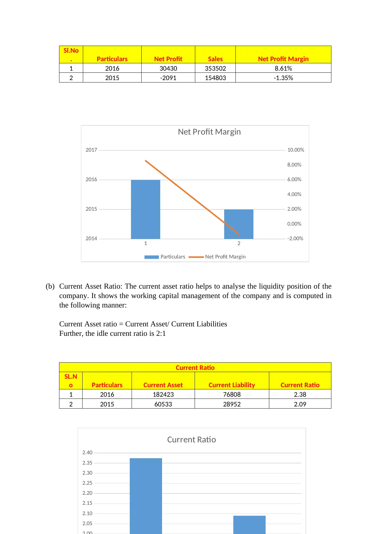
Sl.No
. Particulars Net Profit Sales Net Profit Margin
1 2016 30430 353502 8.61%
2 2015 -2091 154803 -1.35%
(b) Current Asset Ratio: The current asset ratio helps to analyse the liquidity position of the
company. It shows the working capital management of the company and is computed in
the following manner:
Current Asset ratio = Current Asset/ Current Liabilities
Further, the idle current ratio is 2:1
Current Ratio
SL.N
o Particulars Current Asset Current Liability Current Ratio
1 2016 182423 76808 2.38
2 2015 60533 28952 2.09
1 2
2014
2015
2016
2017
-2.00%
0.00%
2.00%
4.00%
6.00%
8.00%
10.00%
Net Profit Margin
Particulars Net Profit Margin
2.05
2.10
2.15
2.20
2.25
2.30
2.35
2.40
Current Ratio
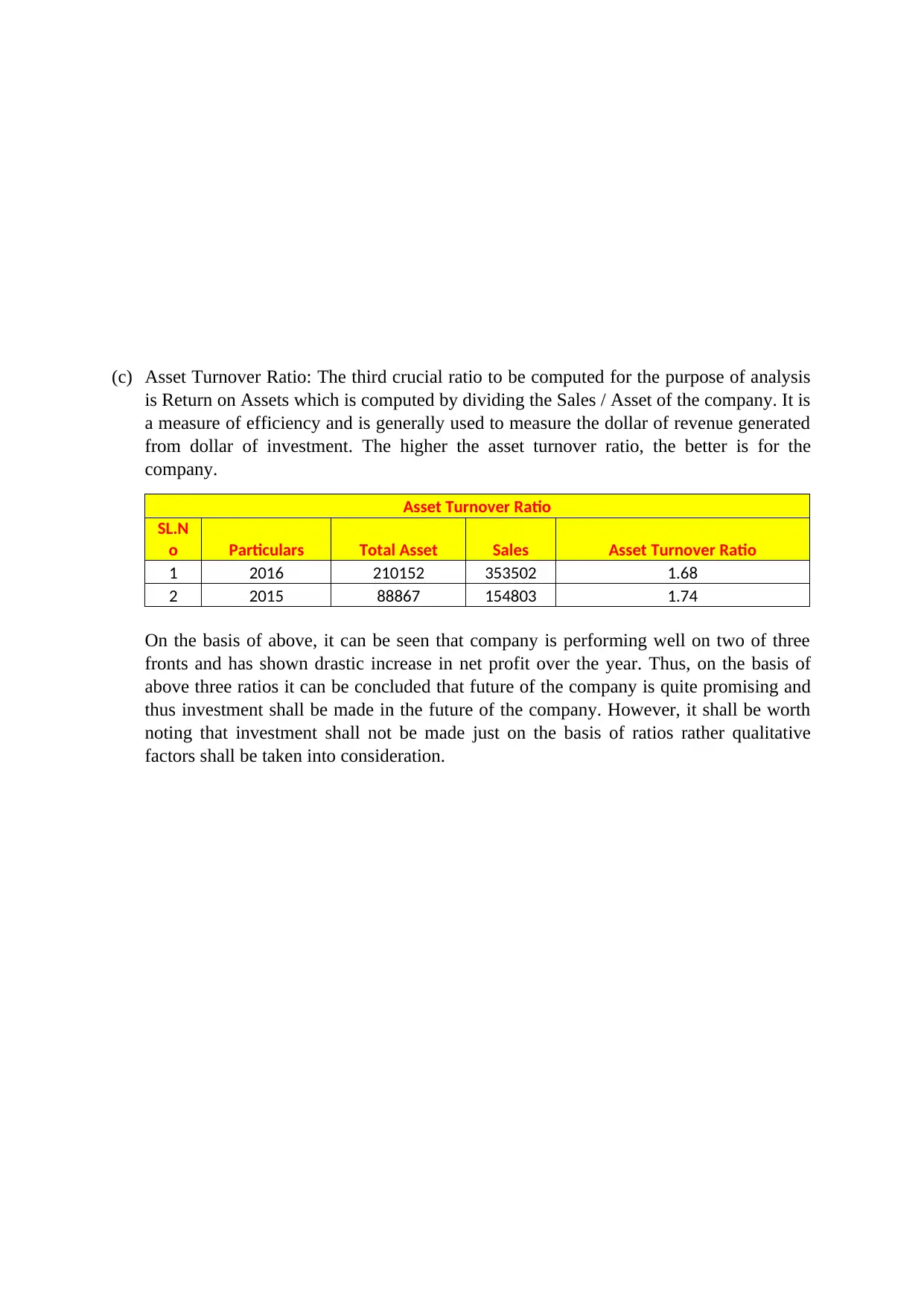
(c) Asset Turnover Ratio: The third crucial ratio to be computed for the purpose of analysis
is Return on Assets which is computed by dividing the Sales / Asset of the company. It is
a measure of efficiency and is generally used to measure the dollar of revenue generated
from dollar of investment. The higher the asset turnover ratio, the better is for the
company.
Asset Turnover Ratio
SL.N
o Particulars Total Asset Sales Asset Turnover Ratio
1 2016 210152 353502 1.68
2 2015 88867 154803 1.74
On the basis of above, it can be seen that company is performing well on two of three
fronts and has shown drastic increase in net profit over the year. Thus, on the basis of
above three ratios it can be concluded that future of the company is quite promising and
thus investment shall be made in the future of the company. However, it shall be worth
noting that investment shall not be made just on the basis of ratios rather qualitative
factors shall be taken into consideration.
2016 2015
1.90
1.95
1 out of 9
Your All-in-One AI-Powered Toolkit for Academic Success.
+13062052269
info@desklib.com
Available 24*7 on WhatsApp / Email
![[object Object]](/_next/static/media/star-bottom.7253800d.svg)
Unlock your academic potential
© 2024 | Zucol Services PVT LTD | All rights reserved.

