Supply Chain Analytics

This document discusses the concept of supply chain analytics and its applications in forecasting and trend analysis. It explains the methods of moving average, regression, and multiplicative decomposition in detail. The document also provides examples and calculations to illustrate the use of these methods.

Running head: SUPPLY CHAIN ANALYTICS
Supply Chain Analytics
Name of the Student:
Name of the University:
Author’s Note:

1SUPPLY CHAIN ANALYTICS
Contents
Answer 1:.........................................................................................................................................2
Answer 1.1...................................................................................................................................3
Answer 1.2...................................................................................................................................3
Answer 2:.........................................................................................................................................3
Answer 3:.........................................................................................................................................7
Answer 4:.........................................................................................................................................9

2SUPPLY CHAIN ANALYTICS
Answer 1:
Moving Average is a technique to calculate overall trend in a data set specially used to
forecast the short term trends. It is calculated by the average of a set of data of specific time
limit. This is known as “Moving” as a new value is generated for the next time period, the oldest
data is neglected. This method removes the irregularities or fluctuations from the data. This is
also known as Simple Moving Average.
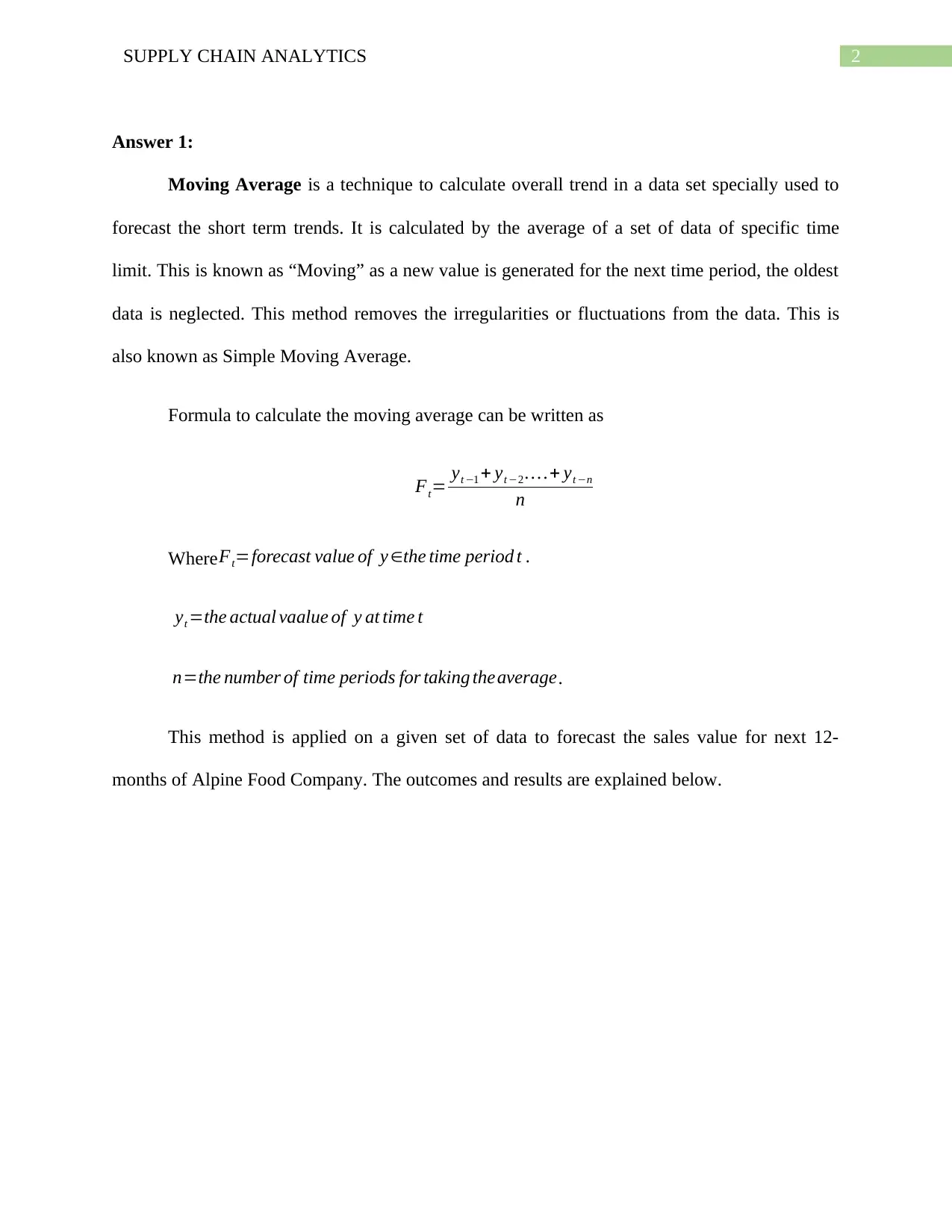
Formula to calculate the moving average can be written as
Ft= yt −1 + yt −2 … .+ yt −n
n
Where Ft=forecast value of y ∈the time period t .
yt =the actual vaalue of y at time t
n=the number of time periods for taking theaverage.
This method is applied on a given set of data to forecast the sales value for next 12-
months of Alpine Food Company. The outcomes and results are explained below.

3SUPPLY CHAIN ANALYTICS
Jan
Feb
Mar
Apr
May
Jun
Jul
Aug
Sep
Oct
Nov
Dec
Jan
Feb
Mar
Apr
May
Jun
Jul
Aug
Sep
Oct
Nov
Dec
Jan
Feb
Mar
Apr
May
Jun
Jul
Aug
Sep
Oct
Nov
Dec
Y1 Y2 Y3
0
50
100
150
200
250
300
350
400
450
500
Actual Vs 12-Months Moving Average
Sales ($ 1000s) of Y1 12-months moving average
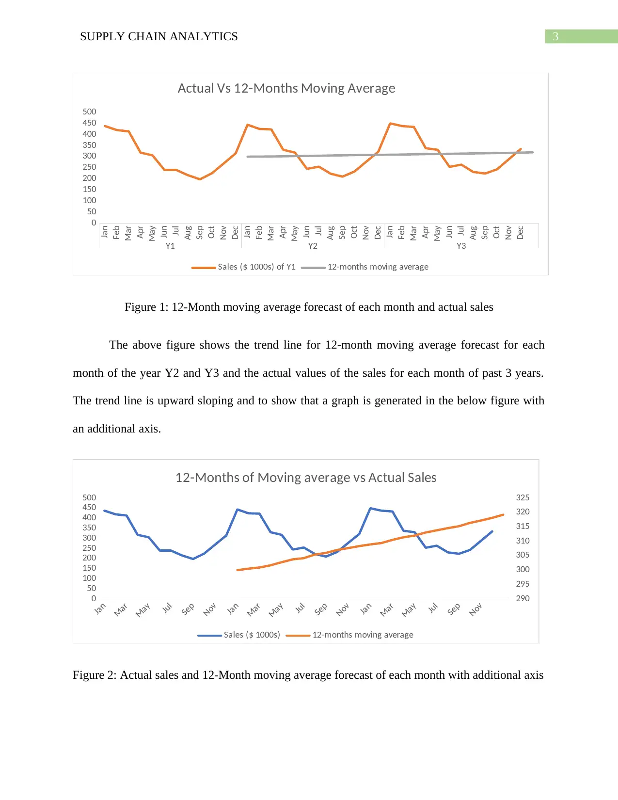
Figure 1: 12-Month moving average forecast of each month and actual sales
The above figure shows the trend line for 12-month moving average forecast for each
month of the year Y2 and Y3 and the actual values of the sales for each month of past 3 years.
The trend line is upward sloping and to show that a graph is generated in the below figure with
an additional axis.
Jan
Mar
May
Jul
Sep
Nov
Jan
Mar
May
Jul
Sep
Nov
Jan
Mar
May
Jul
Sep
Nov
0
50
100
150
200
250
300
350
400
450
500
290
295
300
305
310
315
320
325
12-Months of Moving average vs Actual Sales
Sales ($ 1000s) 12-months moving average
Figure 2: Actual sales and 12-Month moving average forecast of each month with additional axis

4SUPPLY CHAIN ANALYTICS
Answer 1.1
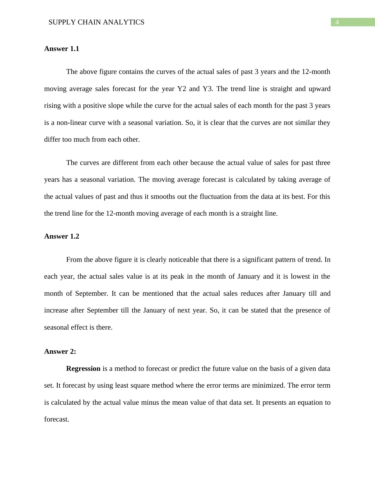
The above figure contains the curves of the actual sales of past 3 years and the 12-month
moving average sales forecast for the year Y2 and Y3. The trend line is straight and upward
rising with a positive slope while the curve for the actual sales of each month for the past 3 years
is a non-linear curve with a seasonal variation. So, it is clear that the curves are not similar they
differ too much from each other.
The curves are different from each other because the actual value of sales for past three
years has a seasonal variation. The moving average forecast is calculated by taking average of
the actual values of past and thus it smooths out the fluctuation from the data at its best. For this
the trend line for the 12-month moving average of each month is a straight line.
Answer 1.2
From the above figure it is clearly noticeable that there is a significant pattern of trend. In
each year, the actual sales value is at its peak in the month of January and it is lowest in the
month of September. It can be mentioned that the actual sales reduces after January till and
increase after September till the January of next year. So, it can be stated that the presence of
seasonal effect is there.
Answer 2:
Regression is a method to forecast or predict the future value on the basis of a given data
set. It forecast by using least square method where the error terms are minimized. The error term
is calculated by the actual value minus the mean value of that data set. It presents an equation to
forecast.

5SUPPLY CHAIN ANALYTICS
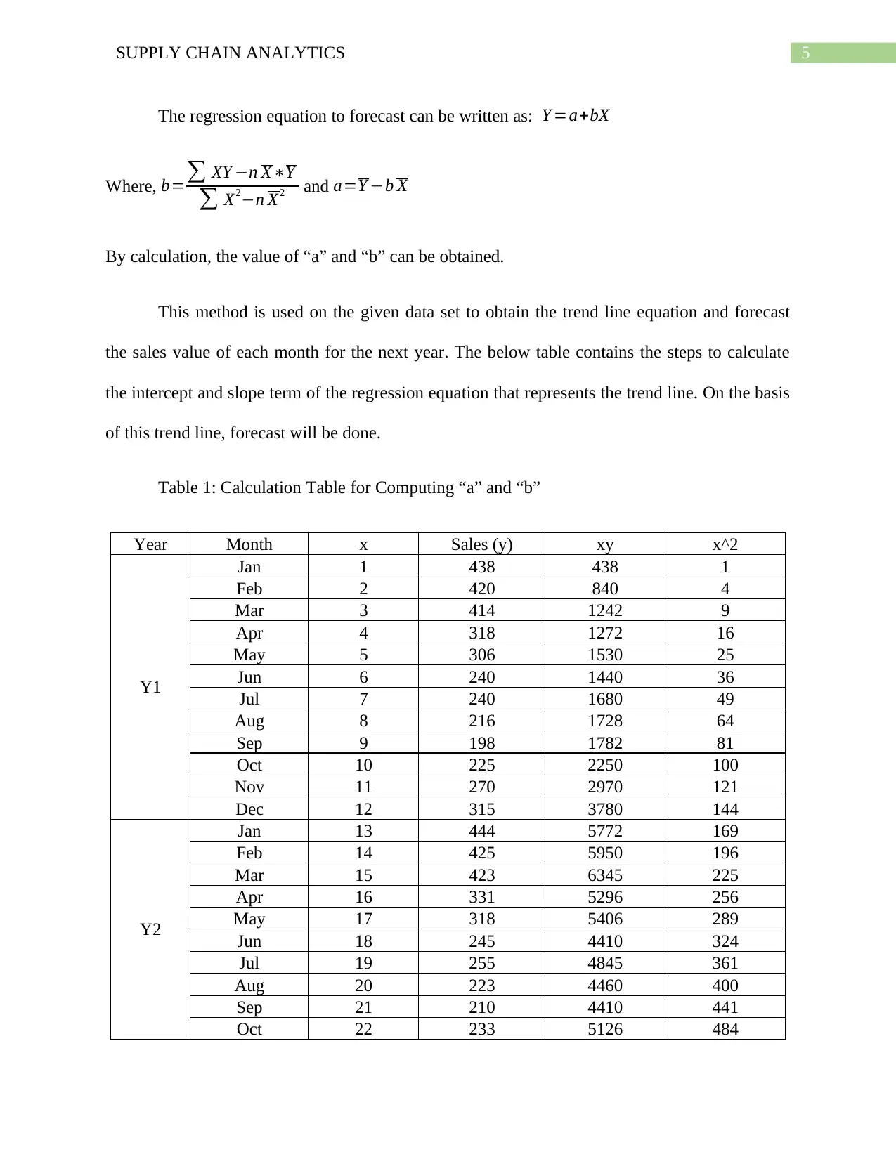
The regression equation to forecast can be written as: Y =a+bX
Where, b=∑ XY −n X∗Y
∑ X2−n X2 and a=Y −b X
By calculation, the value of “a” and “b” can be obtained.
This method is used on the given data set to obtain the trend line equation and forecast
the sales value of each month for the next year. The below table contains the steps to calculate
the intercept and slope term of the regression equation that represents the trend line. On the basis
of this trend line, forecast will be done.
Table 1: Calculation Table for Computing “a” and “b”
Year Month x Sales (y) xy x^2
Y1
Jan 1 438 438 1
Feb 2 420 840 4
Mar 3 414 1242 9
Apr 4 318 1272 16
May 5 306 1530 25
Jun 6 240 1440 36
Jul 7 240 1680 49
Aug 8 216 1728 64
Sep 9 198 1782 81
Oct 10 225 2250 100
Nov 11 270 2970 121
Dec 12 315 3780 144
Y2
Jan 13 444 5772 169
Feb 14 425 5950 196
Mar 15 423 6345 225
Apr 16 331 5296 256
May 17 318 5406 289
Jun 18 245 4410 324
Jul 19 255 4845 361
Aug 20 223 4460 400
Sep 21 210 4410 441
Oct 22 233 5126 484

6SUPPLY CHAIN ANALYTICS
Nov 23 278 6394 529
Dec 24 322 7728 576
Y3
Jan 25 450 11250 625
Feb 26 438 11388 676
Mar 27 434 11718 729
Apr 28 338 9464 784
May 29 331 9599 841
Jun 30 254 7620 900
Jul 31 264 8184 961
Aug 32 231 7392 1024
Sep 33 224 7392 1089
Oct 34 243 8262 1156
Nov 35 289 10115 1225
Dec 36 335 12060 1296
Total 666 11138 201538 16206
Average 18.5 309.3888889 5598.277778 450.1666667
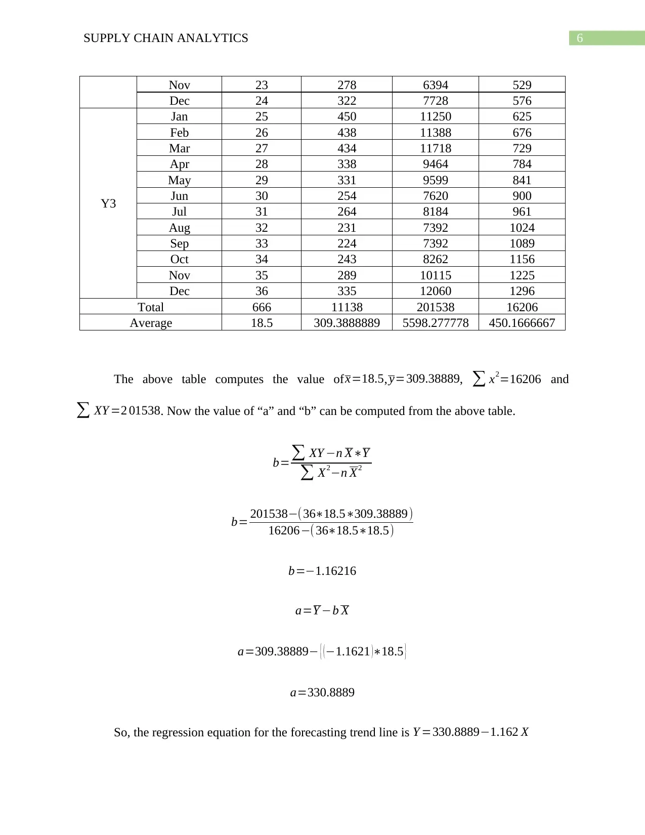
The above table computes the value of x=18.5, y=309.38889, ∑ x2=16206 and
∑ XY =2 01538. Now the value of “a” and “b” can be computed from the above table.
b=∑ XY −n X∗Y
∑ X2−n X2
b= 201538−(36∗18.5∗309.38889)
16206−( 36∗18.5∗18.5)
b=−1.16216
a=Y −b X
a=309.38889− { ( −1.1621 )∗18.5 }
a=330.8889
So, the regression equation for the forecasting trend line is Y =330.8889−1.162 X

7SUPPLY CHAIN ANALYTICS
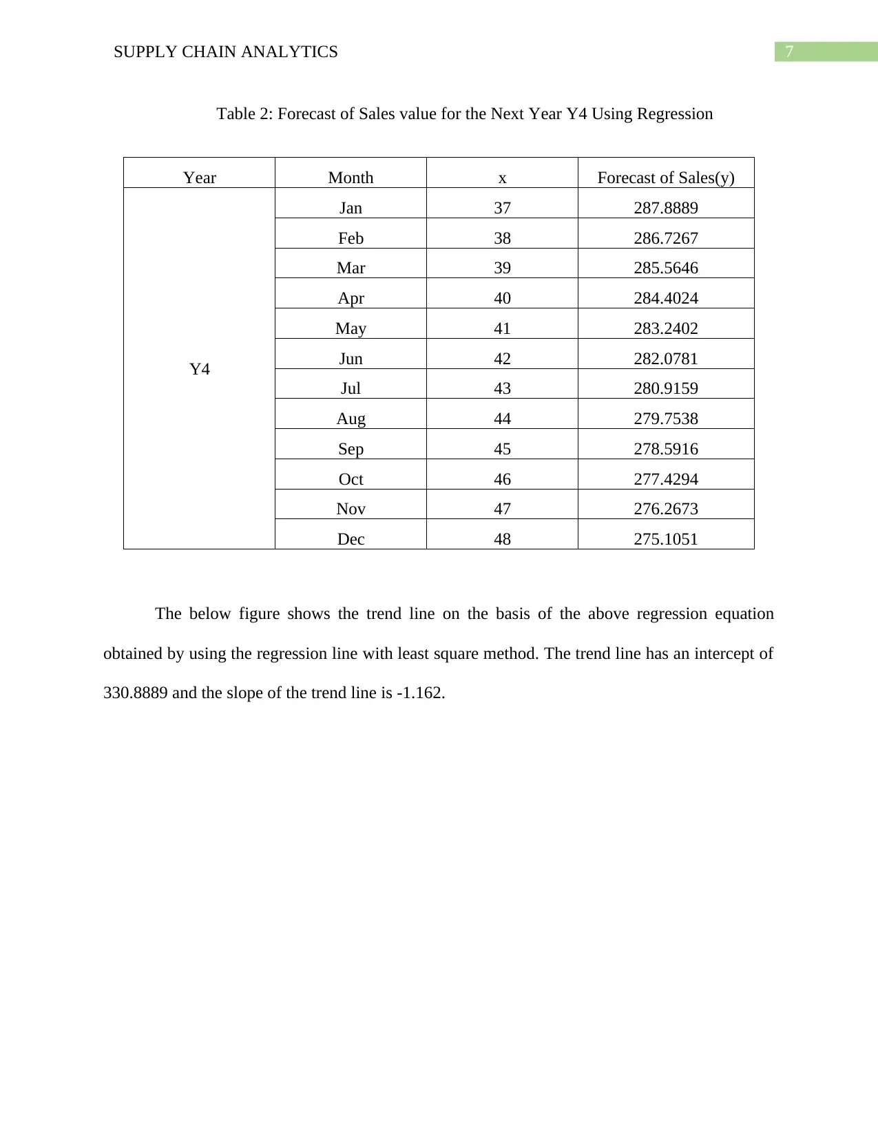
Table 2: Forecast of Sales value for the Next Year Y4 Using Regression
Year Month x Forecast of Sales(y)
Y4
Jan 37 287.8889
Feb 38 286.7267
Mar 39 285.5646
Apr 40 284.4024
May 41 283.2402
Jun 42 282.0781
Jul 43 280.9159
Aug 44 279.7538
Sep 45 278.5916
Oct 46 277.4294
Nov 47 276.2673
Dec 48 275.1051
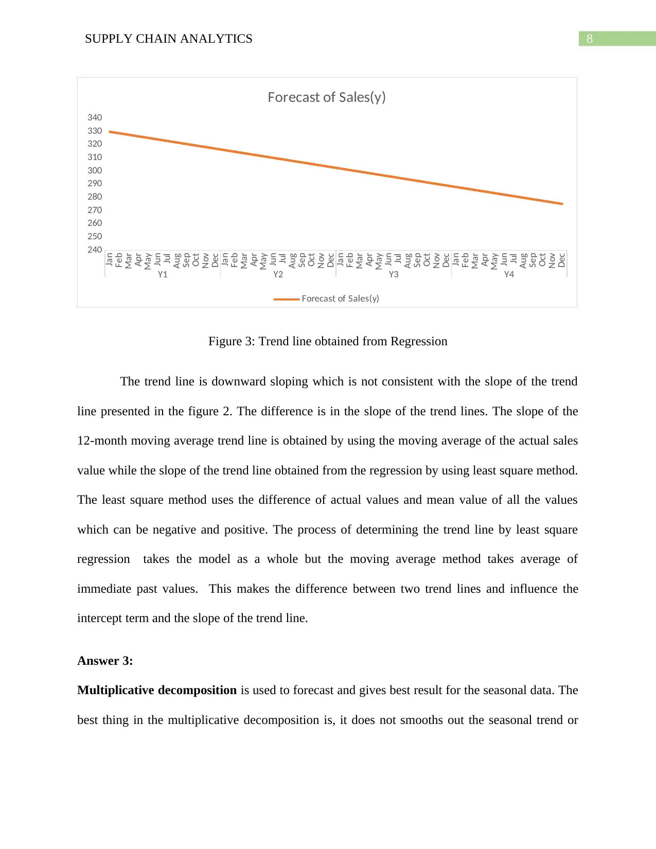
The below figure shows the trend line on the basis of the above regression equation
obtained by using the regression line with least square method. The trend line has an intercept of
330.8889 and the slope of the trend line is -1.162.

8SUPPLY CHAIN ANALYTICS
Jan
Feb
Mar
Apr
May
Jun
Jul
Aug
Sep
Oct
Nov
Dec
Jan
Feb
Mar
Apr
May
Jun
Jul
Aug
Sep
Oct
Nov
Dec
Jan
Feb
Mar
Apr
May
Jun
Jul
Aug
Sep
Oct
Nov
Dec
Jan
Feb
Mar
Apr
May
Jun
Jul
Aug
Sep
Oct
Nov
Dec
Y1 Y2 Y3 Y4
240
250
260
270
280
290
300
310
320
330
340
Forecast of Sales(y)
Forecast of Sales(y)
Figure 3: Trend line obtained from Regression
The trend line is downward sloping which is not consistent with the slope of the trend
line presented in the figure 2. The difference is in the slope of the trend lines. The slope of the
12-month moving average trend line is obtained by using the moving average of the actual sales
value while the slope of the trend line obtained from the regression by using least square method.
The least square method uses the difference of actual values and mean value of all the values
which can be negative and positive. The process of determining the trend line by least square
regression takes the model as a whole but the moving average method takes average of
immediate past values. This makes the difference between two trend lines and influence the
intercept term and the slope of the trend line.
Answer 3:
Multiplicative decomposition is used to forecast and gives best result for the seasonal data. The
best thing in the multiplicative decomposition is, it does not smooths out the seasonal trend or

9SUPPLY CHAIN ANALYTICS
fluctuations due to seasonal trend. It considers the seasonal trend and thus reduces the absolute
error to forecast more effectively.
Month
Jan
Feb
Mar
Apr
May
Jun
Jul
Aug
Sep
Oct
Nov
Dec
Jan
Feb
Mar
Apr
May
Jun
Jul
Aug
Sep
Oct
Nov
Dec
Jan
Feb
Mar
Apr
May
Jun
Jul
Aug
Sep
Oct
Nov
Dec
Jan
Feb
Mar
Apr
May
Jun
Jul
Aug
Sep
Oct
Nov
Dec
Y
e
ar
Y1 Y2 Y3 Y4
0.00
50.00
100.00
150.00
200.00
250.00
300.00
350.00
400.00
450.00
500.00
Forecast Computed by Multiplicative Decomposition
Forecast
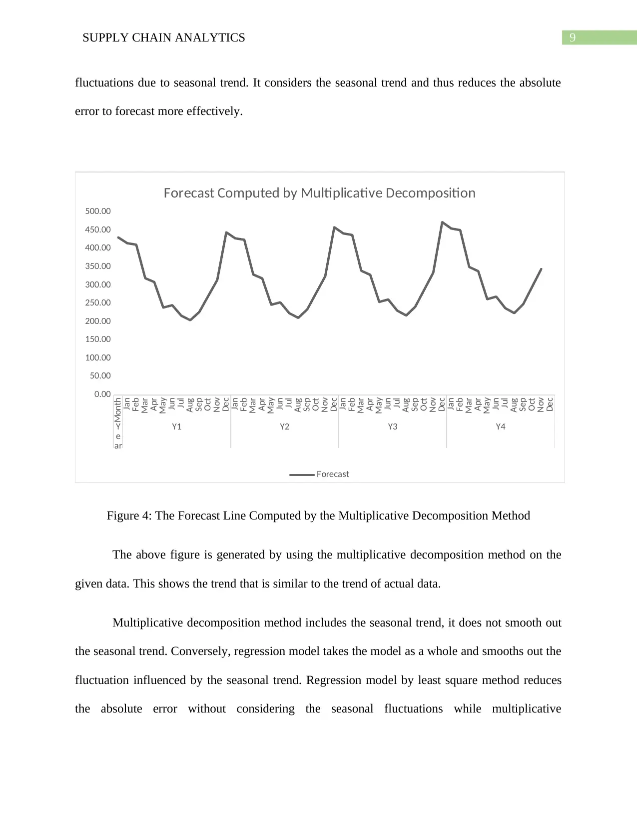
Figure 4: The Forecast Line Computed by the Multiplicative Decomposition Method
The above figure is generated by using the multiplicative decomposition method on the
given data. This shows the trend that is similar to the trend of actual data.
Multiplicative decomposition method includes the seasonal trend, it does not smooth out
the seasonal trend. Conversely, regression model takes the model as a whole and smooths out the
fluctuation influenced by the seasonal trend. Regression model by least square method reduces
the absolute error without considering the seasonal fluctuations while multiplicative

10SUPPLY CHAIN ANALYTICS
decomposition takes care of the seasonal fluctuation and does not neutralize it while forecasting
which gives the better result for each month and does not predict too much or too less.
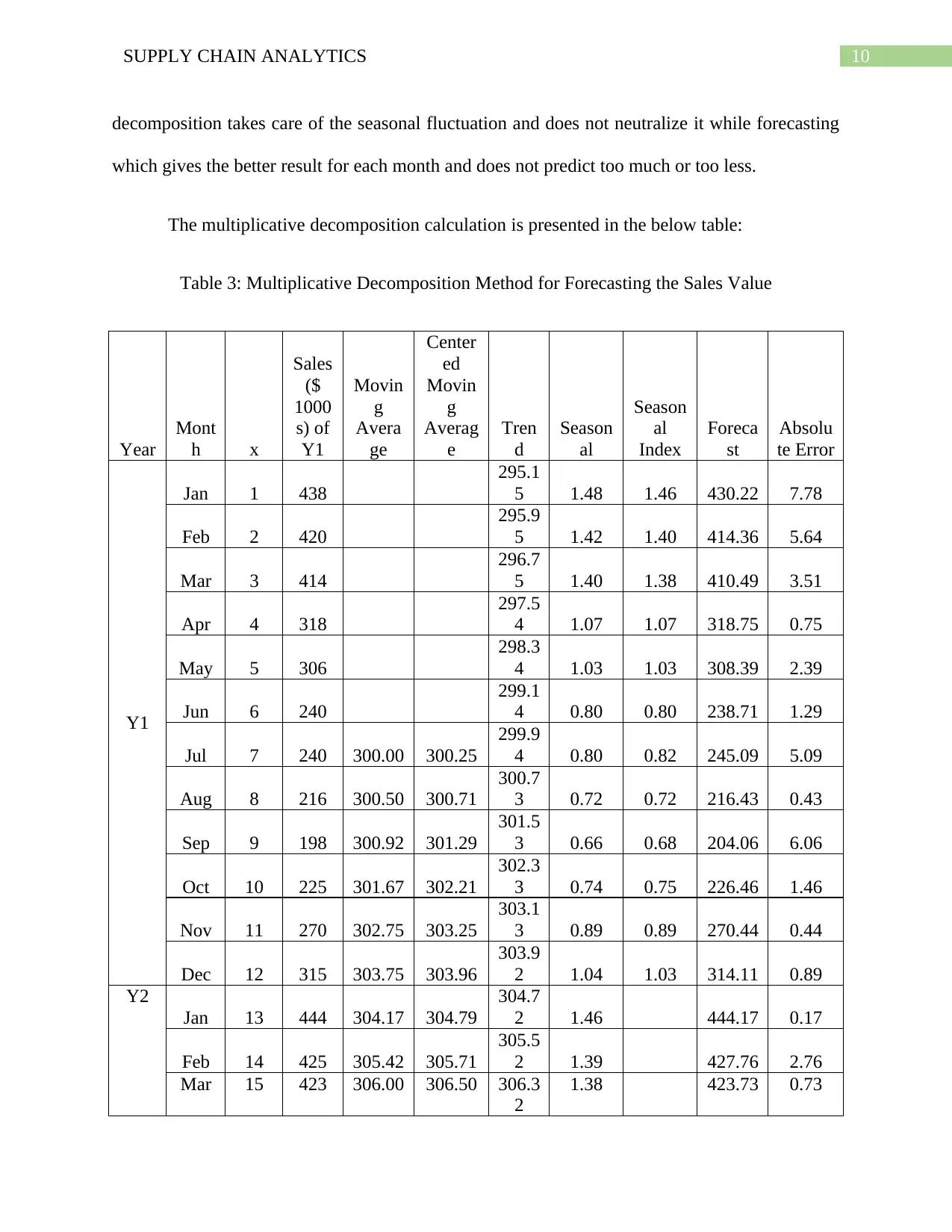
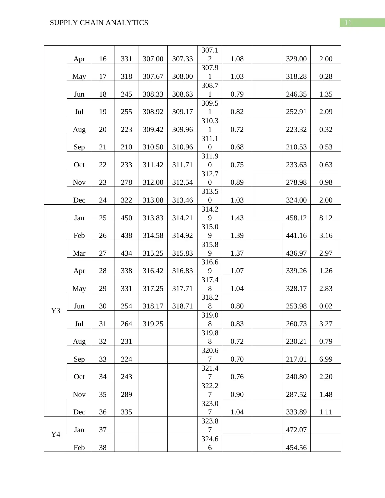
The multiplicative decomposition calculation is presented in the below table:
Table 3: Multiplicative Decomposition Method for Forecasting the Sales Value
Year
Mont
h x
Sales
($
1000
s) of
Y1
Movin
g
Avera
ge
Center
ed
Movin
g
Averag
e
Tren
d
Season
al
Season
al
Index
Foreca
st
Absolu
te Error
Y1
Jan 1 438
295.1
5 1.48 1.46 430.22 7.78
Feb 2 420
295.9
5 1.42 1.40 414.36 5.64
Mar 3 414
296.7
5 1.40 1.38 410.49 3.51
Apr 4 318
297.5
4 1.07 1.07 318.75 0.75
May 5 306
298.3
4 1.03 1.03 308.39 2.39
Jun 6 240
299.1
4 0.80 0.80 238.71 1.29
Jul 7 240 300.00 300.25
299.9
4 0.80 0.82 245.09 5.09
Aug 8 216 300.50 300.71
300.7
3 0.72 0.72 216.43 0.43
Sep 9 198 300.92 301.29
301.5
3 0.66 0.68 204.06 6.06
Oct 10 225 301.67 302.21
302.3
3 0.74 0.75 226.46 1.46
Nov 11 270 302.75 303.25
303.1
3 0.89 0.89 270.44 0.44
Dec 12 315 303.75 303.96
303.9
2 1.04 1.03 314.11 0.89
Y2
Jan 13 444 304.17 304.79
304.7
2 1.46 444.17 0.17
Feb 14 425 305.42 305.71
305.5
2 1.39 427.76 2.76
Mar 15 423 306.00 306.50 306.3
2
1.38 423.73 0.73

11SUPPLY CHAIN ANALYTICS
Apr 16 331 307.00 307.33
307.1
2 1.08 329.00 2.00
May 17 318 307.67 308.00
307.9
1 1.03 318.28 0.28
Jun 18 245 308.33 308.63
308.7
1 0.79 246.35 1.35
Jul 19 255 308.92 309.17
309.5
1 0.82 252.91 2.09
Aug 20 223 309.42 309.96
310.3
1 0.72 223.32 0.32
Sep 21 210 310.50 310.96
311.1
0 0.68 210.53 0.53
Oct 22 233 311.42 311.71
311.9
0 0.75 233.63 0.63
Nov 23 278 312.00 312.54
312.7
0 0.89 278.98 0.98
Dec 24 322 313.08 313.46
313.5
0 1.03 324.00 2.00
Y3
Jan 25 450 313.83 314.21
314.2
9 1.43 458.12 8.12
Feb 26 438 314.58 314.92
315.0
9 1.39 441.16 3.16
Mar 27 434 315.25 315.83
315.8
9 1.37 436.97 2.97
Apr 28 338 316.42 316.83
316.6
9 1.07 339.26 1.26
May 29 331 317.25 317.71
317.4
8 1.04 328.17 2.83
Jun 30 254 318.17 318.71
318.2
8 0.80 253.98 0.02
Jul 31 264 319.25
319.0
8 0.83 260.73 3.27
Aug 32 231
319.8
8 0.72 230.21 0.79
Sep 33 224
320.6
7 0.70 217.01 6.99
Oct 34 243
321.4
7 0.76 240.80 2.20
Nov 35 289
322.2
7 0.90 287.52 1.48
Dec 36 335
323.0
7 1.04 333.89 1.11
Y4 Jan 37
323.8
7 472.07
Feb 38
324.6
6 454.56

12SUPPLY CHAIN ANALYTICS
Mar 39
325.4
6 450.22
Apr 40
326.2
6 349.51
May 41
327.0
6 338.07
Jun 42
327.8
5 261.62
Jul 43
328.6
5 268.56
Aug 44
329.4
5 237.10
Sep 45
330.2
5 223.49
Oct 46
331.0
4 247.97
Nov 47
331.8
4 296.06
Dec 48
332.6
4 343.78
Answer 4:
Jan
Feb
Mar
Apr
May
Jun
Jul
Aug
Sep
Oct
Nov
Dec
Jan
Feb
Mar
Apr
May
Jun
Jul
Aug
Sep
Oct
Nov
Dec
Jan
Feb
Mar
Apr
May
Jun
Jul
Aug
Sep
Oct
Nov
Dec
Jan
Feb
Mar
Apr
May
Jun
Jul
Aug
Sep
Oct
Nov
Dec
Y1 Y2 Y3 Y4
0
50
100
150
200
250
300
350
400
450
500
Comparision of Forecast
Sales ($ 1000s) of Y1 12-months moving average Forecast of Sales
Regression Forecast of Sales MD Forecast of Sales
Figure 5: Comparison of Forecast Generated by Different Methods

13SUPPLY CHAIN ANALYTICS
The above figure shows the forecast trend lines generated by the methods like the 12-
months moving average, regression and the multiplicative decomposition. The straight line
trends are generated by the regression and 12-months mobbing average method that are not able
to forecast significantly. But the forecast obtained from the multiplicative decomposition method
is partially overlapping on the actual sales line which means the forecast is robust and can be
predictable by the forecast line obtained by the multiplicative decomposition method. So, it is
better to use the multiplicative decomposition method to forecast the sales of each month of
Alpine Food Company. Another statistics is absolute error for the three methods can explain
which is better for forecasting. The 12-month moving average has average absolute error of -
5.375, the regression method has average absolute error of 67.69 and the multiplicative
decomposition has average absolute error of 2.33. The least error gives the best result. So, it can
be concluded that the multiplicative decomposition is the best method to forecast the sales value
for each month of next year.