Statistics Assignment: Hypothesis Testing, Regression Analysis, ANOVA

Verified

Added on  2021/06/18

|10
|1143
|162
Homework Assignment
AI Summary
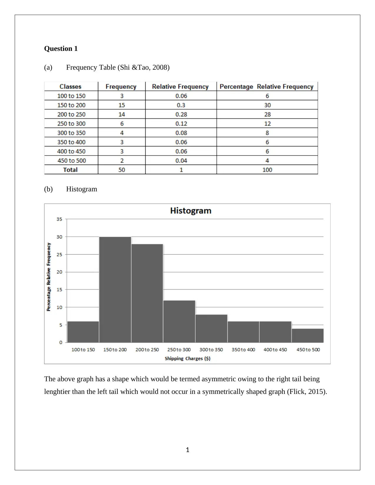
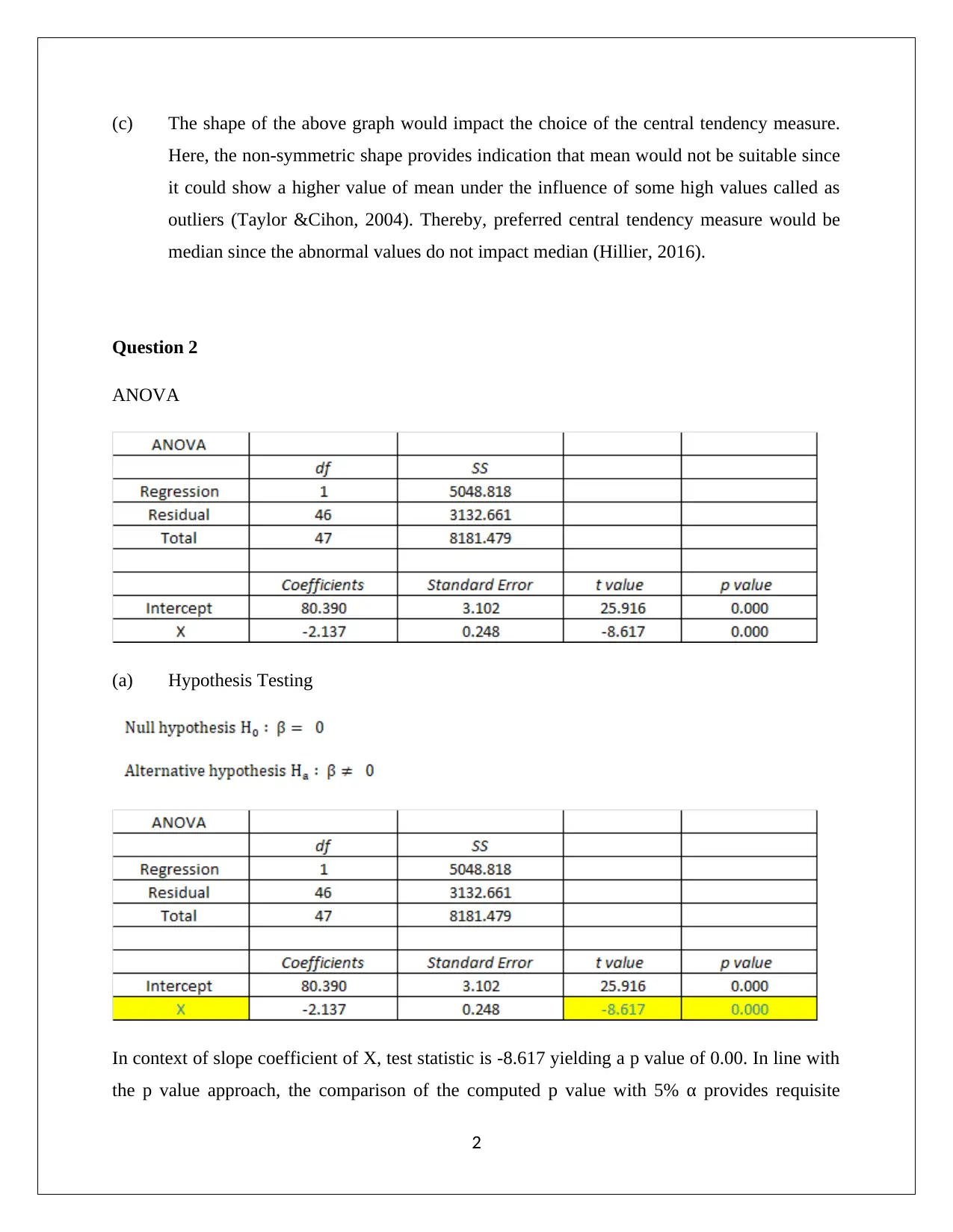
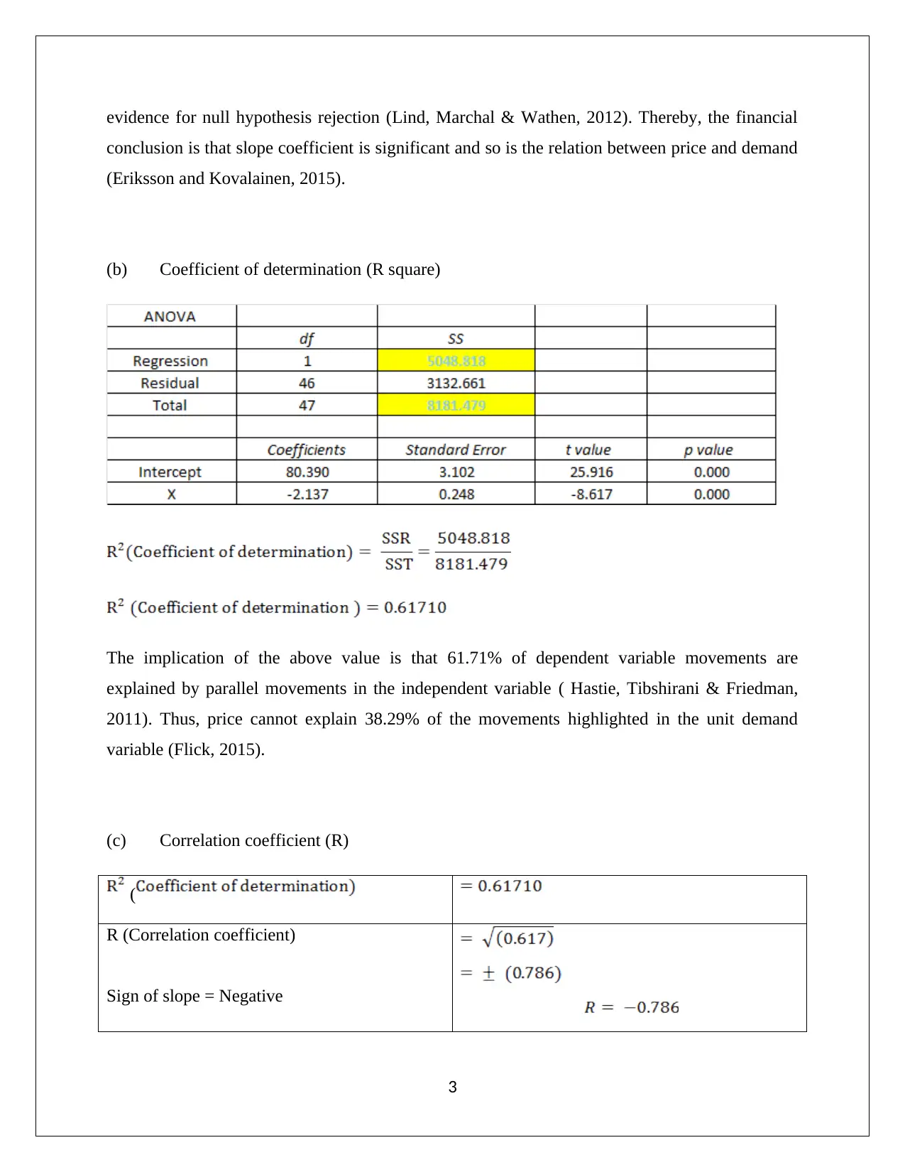
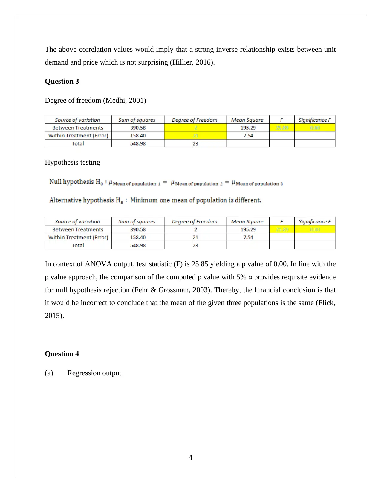
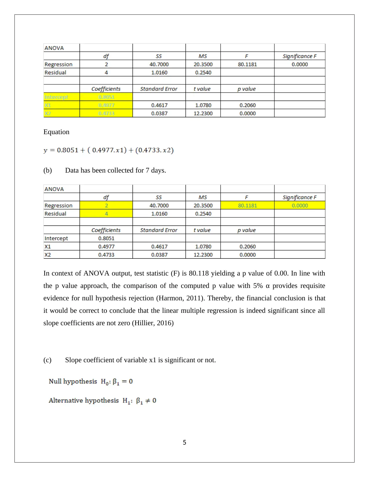
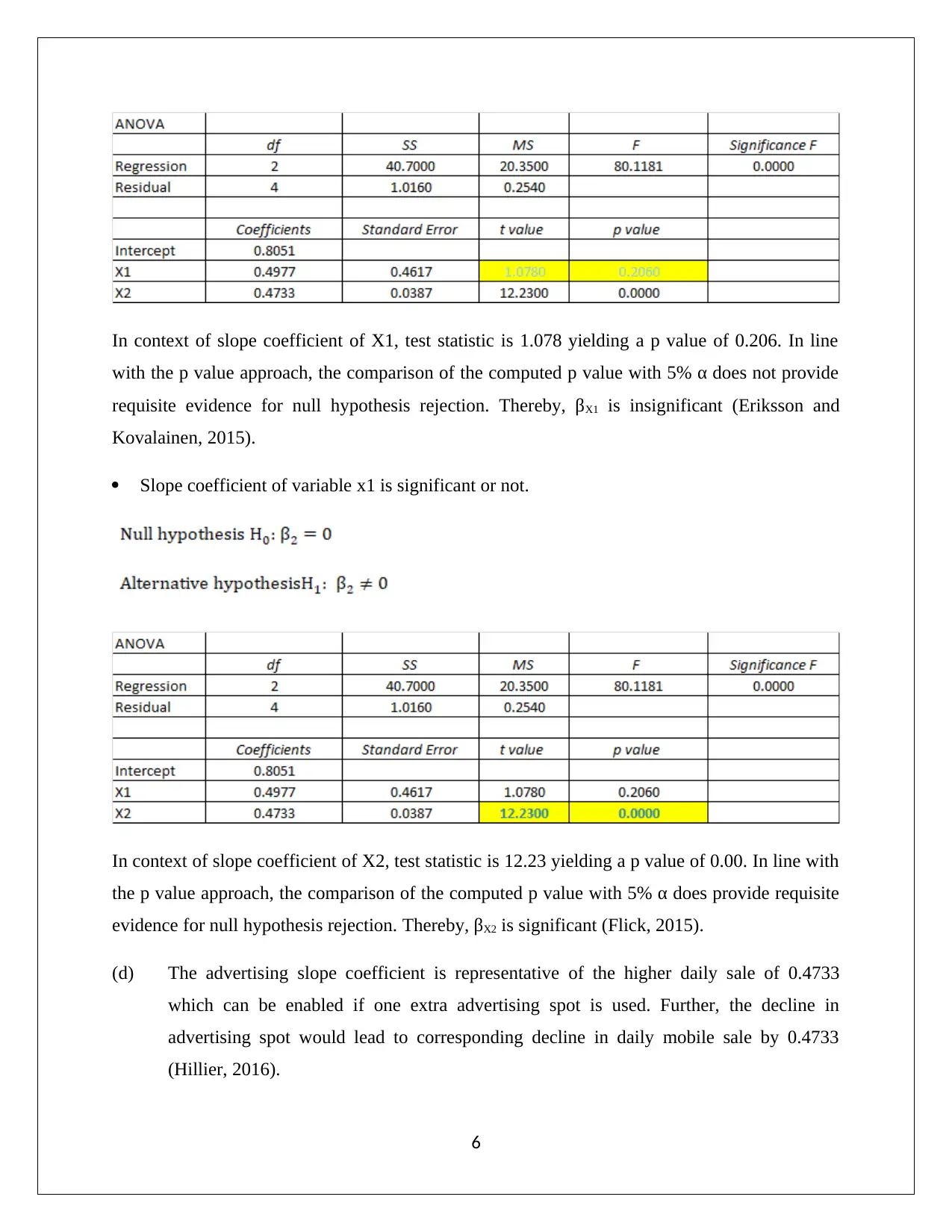
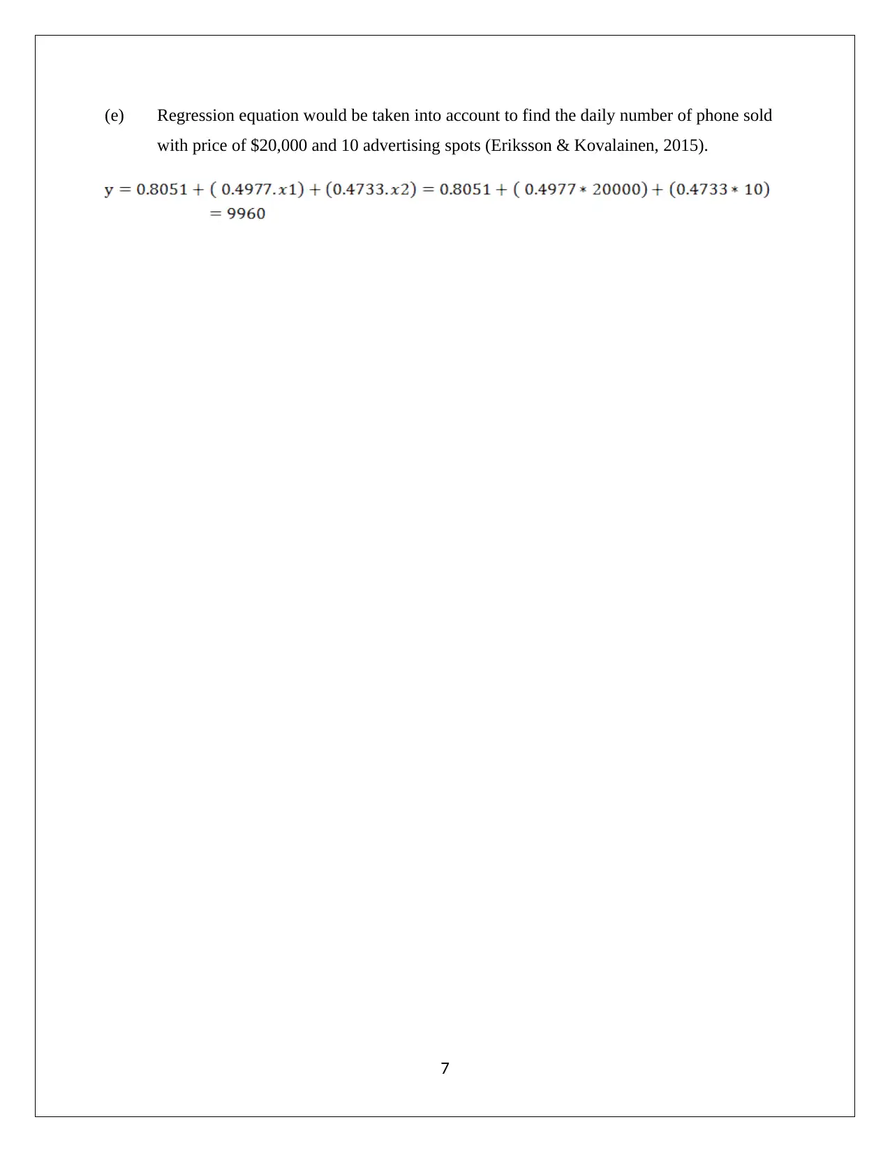
This statistics assignment solution addresses several key statistical concepts. It begins with an analysis of a frequency table and histogram, discussing the shape of the graph and its impact on the choice of central tendency measures, specifically arguing for the use of the median due to the presence of outliers. The solution then proceeds to an ANOVA analysis, including hypothesis testing, and interpretation of the results. Further, the assignment delves into regression analysis, calculating and interpreting the coefficient of determination (R-squared) and correlation coefficient, and discussing the implications of these values. The solution also covers the degree of freedom in hypothesis testing using ANOVA and interpreting the F-statistic and p-value. The final part of the assignment explores multiple linear regression, including the development of a regression equation, and the interpretation of slope coefficients, with specific reference to advertising's impact on sales. The assignment provides detailed calculations, interpretations, and financial conclusions for each question, referencing relevant statistical literature.
Document Page
Statistics
Assignment
Student Name
[Pick the date]
tabler-icon-diamond-filled.svg

Paraphrase This Document

Need a fresh take? Get an instant paraphrase of this document with our AI Paraphraser
Document Page
Question 1
(a) Frequency Table (Shi &Tao, 2008)
(b) Histogram
The above graph has a shape which would be termed asymmetric owing to the right tail being
lenghtier than the left tail which would not occur in a symmetrically shaped graph (Flick, 2015).
1
Document Page
(c) The shape of the above graph would impact the choice of the central tendency measure.
Here, the non-symmetric shape provides indication that mean would not be suitable since
it could show a higher value of mean under the influence of some high values called as
outliers (Taylor &Cihon, 2004). Thereby, preferred central tendency measure would be
median since the abnormal values do not impact median (Hillier, 2016).
Question 2
ANOVA
(a) Hypothesis Testing
In context of slope coefficient of X, test statistic is -8.617 yielding a p value of 0.00. In line with
the p value approach, the comparison of the computed p value with 5% α provides requisite
2
Document Page
evidence for null hypothesis rejection (Lind, Marchal & Wathen, 2012). Thereby, the financial
conclusion is that slope coefficient is significant and so is the relation between price and demand
(Eriksson and Kovalainen, 2015).
(b) Coefficient of determination (R square)
The implication of the above value is that 61.71% of dependent variable movements are
explained by parallel movements in the independent variable ( Hastie, Tibshirani & Friedman,
2011). Thus, price cannot explain 38.29% of the movements highlighted in the unit demand
variable (Flick, 2015).
(c) Correlation coefficient (R)
(
R (Correlation coefficient)
Sign of slope = Negative
3
tabler-icon-diamond-filled.svg

Paraphrase This Document

Need a fresh take? Get an instant paraphrase of this document with our AI Paraphraser
Document Page
The above correlation values would imply that a strong inverse relationship exists between unit
demand and price which is not surprising (Hillier, 2016).
Question 3
Degree of freedom (Medhi, 2001)
Hypothesis testing
In context of ANOVA output, test statistic (F) is 25.85 yielding a p value of 0.00. In line with the
p value approach, the comparison of the computed p value with 5% α provides requisite evidence
for null hypothesis rejection (Fehr & Grossman, 2003). Thereby, the financial conclusion is that
it would be incorrect to conclude that the mean of the given three populations is the same (Flick,
2015).
Question 4
(a) Regression output
4
Document Page
Equation
(b) Data has been collected for 7 days.
In context of ANOVA output, test statistic (F) is 80.118 yielding a p value of 0.00. In line with
the p value approach, the comparison of the computed p value with 5% α provides requisite
evidence for null hypothesis rejection (Harmon, 2011). Thereby, the financial conclusion is that
it would be correct to conclude that the linear multiple regression is indeed significant since all
slope coefficients are not zero (Hillier, 2016)
(c) Slope coefficient of variable x1 is significant or not.
5
Document Page
In context of slope coefficient of X1, test statistic is 1.078 yielding a p value of 0.206. In line
with the p value approach, the comparison of the computed p value with 5% α does not provide
requisite evidence for null hypothesis rejection. Thereby, βX1 is insignificant (Eriksson and
Kovalainen, 2015).
Slope coefficient of variable x1 is significant or not.
In context of slope coefficient of X2, test statistic is 12.23 yielding a p value of 0.00. In line with
the p value approach, the comparison of the computed p value with 5% α does provide requisite
evidence for null hypothesis rejection. Thereby, βX2 is significant (Flick, 2015).
(d) The advertising slope coefficient is representative of the higher daily sale of 0.4733
which can be enabled if one extra advertising spot is used. Further, the decline in
advertising spot would lead to corresponding decline in daily mobile sale by 0.4733
(Hillier, 2016).
6
tabler-icon-diamond-filled.svg

Paraphrase This Document

Need a fresh take? Get an instant paraphrase of this document with our AI Paraphraser
Document Page
(e) Regression equation would be taken into account to find the daily number of phone sold
with price of $20,000 and 10 advertising spots (Eriksson & Kovalainen, 2015).
7
Document Page
References
Eriksson, P. & Kovalainen, A. (2015) Quantitative methods in business research 3rd ed. London:
Sage Publications.
Fehr, F. H., & Grossman, G. (2003). An introduction to sets, probability and hypothesis testing
(3rd ed.). Ohio: Heath.
Flick, U. (2015) Introducing research methodology: A beginner's guide to doing a research
project. 4th ed. New York: Sage Publications.
Harmon, M. (2011). Hypothesis Testing in Excel - The Excel Statistical Master (7th ed.). Florida:
Mark Harmon.
Hastie, T., Tibshirani, R. & Friedman, J. (2011). The Elements of Statistical Learning (4th
ed.). New York: Springer Publications.
Hillier, F. (2016) Introduction to Operations Research 6th ed. New York: McGraw Hill
Publications.
Lind, A.D., Marchal, G.W. & Wathen, A.S. (2012). Statistical Techniques in Business and
Economics (15th ed.). New York : McGraw-Hill/Irwin.
Medhi, J. (2001). Statistical Methods: An Introductory Text (4th ed.). Sydney: New Age
International.
Shi, Z. N. & Tao, J. (2008). Statistical Hypothesis Testing: Theory and Methods (6th ed.).
London: World Scientific.
Taylor, K. J. & Cihon, C. (2004). Statistical Techniques for Data Analysis (2nd ed.). Melbourne:
CRC Press.
8
Document Page
9
chevron_up_icon
1 out of 10
circle_padding
hide_on_mobile
zoom_out_icon