Synthesis of Sinusoidal Signals-MUS Signal Processing Lab 04

The lab experiment focuses on the music synthesis and sinusoids. The lab seeks to establish a connection between the musical notes and their respective frequencies and sinusoids. The implementation of structure for grouping information in MATLAB scripts results in the output below for the script code snippet attached.

SYNTHESIS OF SINUSOIDAL SIGNALS-
MUSIC SYNTHESIS
SIGNAL PROCESSING LAB 04
STUDENT NAME
STUDENT ID NUMBER
Institutional Affiliation
Location
Instructor (tutor)
Date of submission
12/5/2018

INTRODUCTION
The lab experiment focuses on the music synthesis and sinusoids. There is need to employ great
effort in determining the documented work and MATLAB implementation.
LAB EXPERIMENT: PRE-LAB
PART I: D-TO-A CONVERSION
The songs are extracted from the long list of Beethoven music from the 19th century. One of the
songs considered for this experiment is the “hallelujah”. The music synthesis will be done with
sinusoidal waveforms of the form,
x (t )=∑
k
Ak cos ( ωk t +ϕk )
The lab seeks to establish a connection between the musical notes and their respective
frequencies and sinusoids. This lab seeks to create the periodic waveforms for the music signals
and, thereafter, plays the music via a loudspeaker. There is need to convert the signals from
digital samples to an actual continuous waveform representing actual voltage and the values are
sent to the loudspeaker for analysis. The process requires that the signal is sampled and then
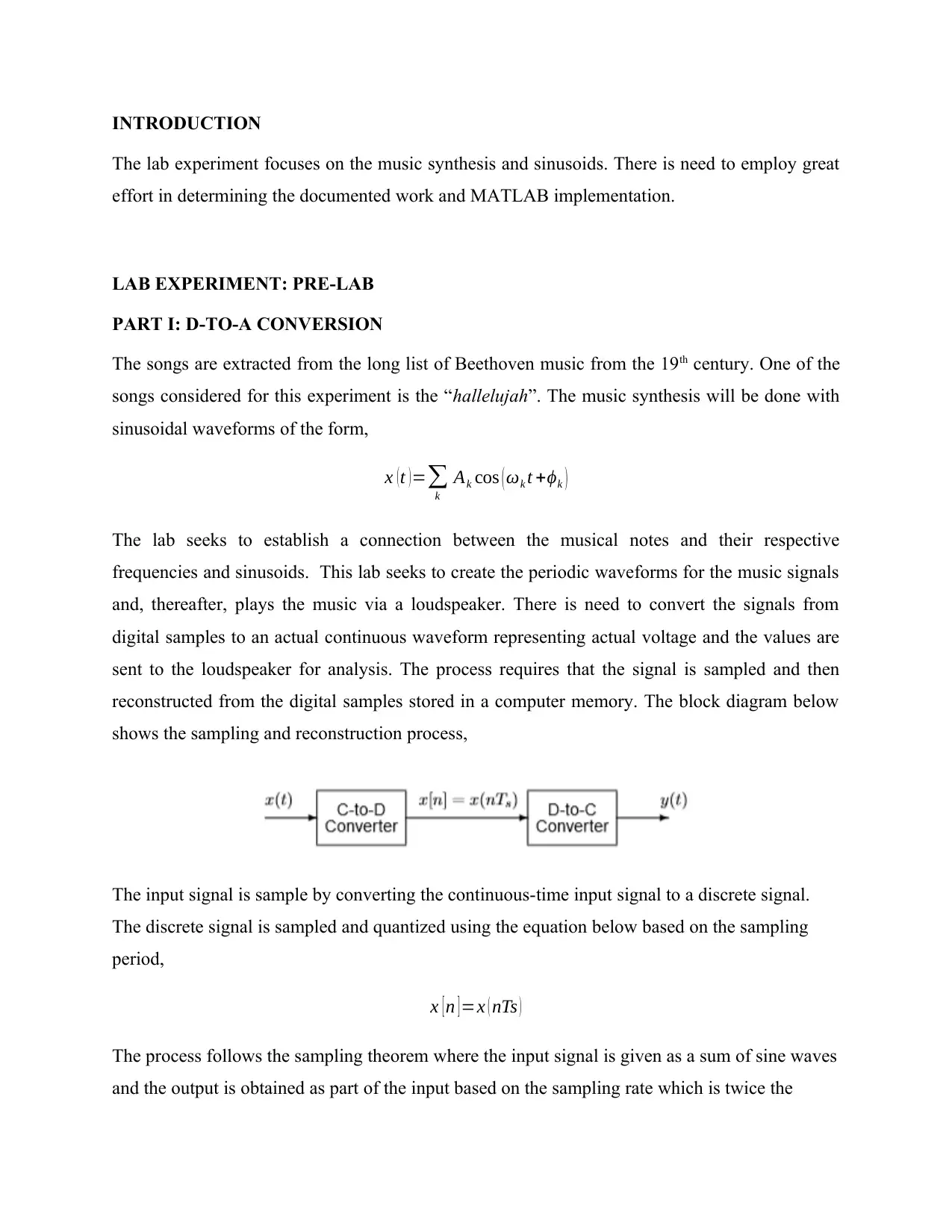
reconstructed from the digital samples stored in a computer memory. The block diagram below
shows the sampling and reconstruction process,
The input signal is sample by converting the continuous-time input signal to a discrete signal.
The discrete signal is sampled and quantized using the equation below based on the sampling
period,
x [ n ] =x ( nTs )
The process follows the sampling theorem where the input signal is given as a sum of sine waves
and the output is obtained as part of the input based on the sampling rate which is twice the

maximum frequency. The theorem is also known as the nyquist theorem. In the block diagram
there are two critical processes namely:
(i) Analog-to-digital converter
(ii) Digital-to-analog converter
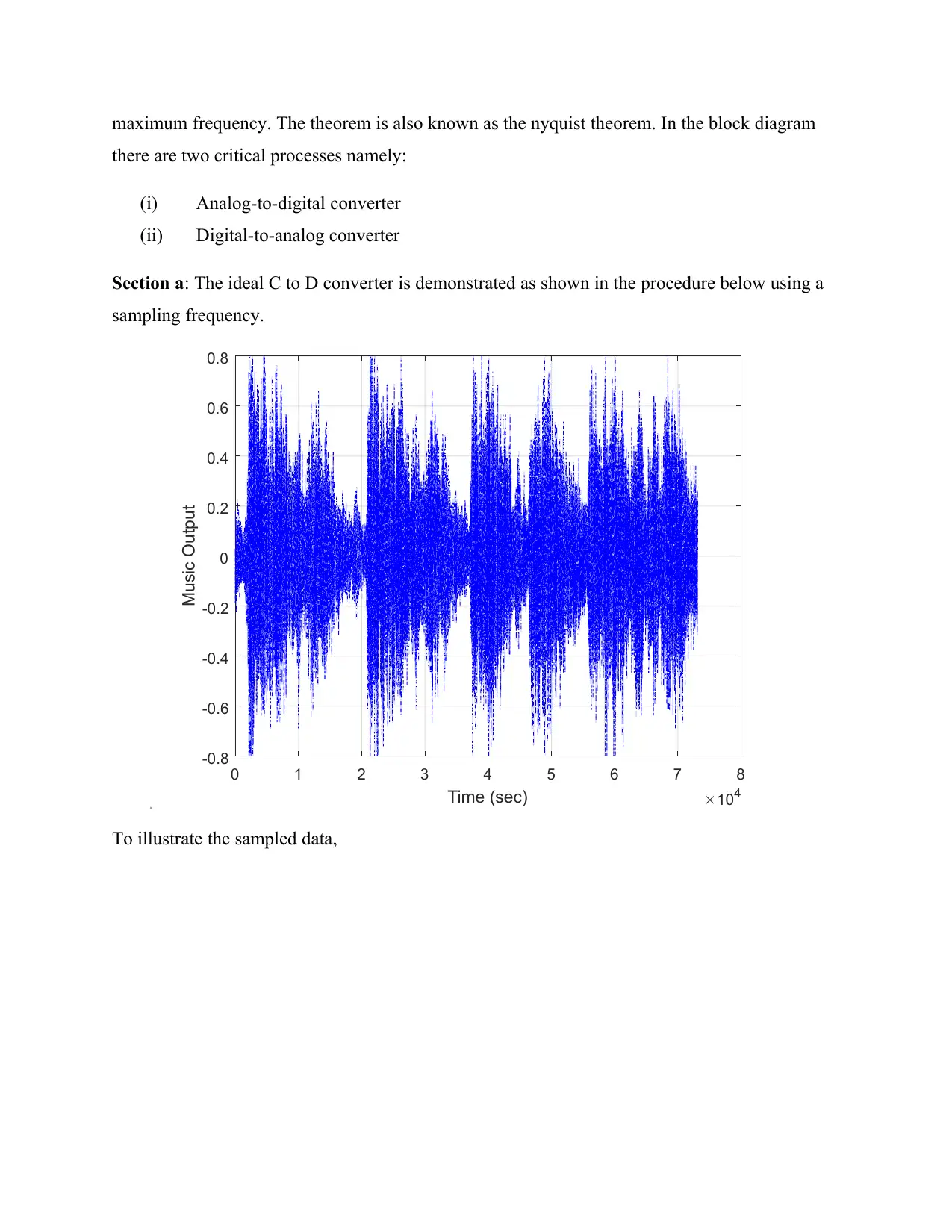
Section a: The ideal C to D converter is demonstrated as shown in the procedure below using a
sampling frequency.
0 1 2 3 4 5 6 7 8
Time (sec) 104
-0.8
-0.6
-0.4
-0.2
0
0.2
0.4
0.6
0.8
Music Output
C to D Converter
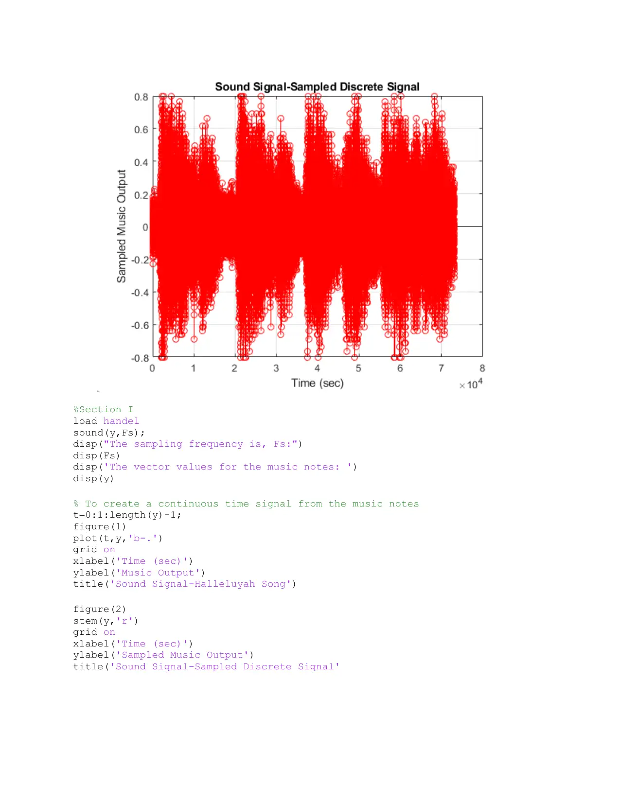
To illustrate the sampled data,

%Section I
load handel
sound(y,Fs);
disp("The sampling frequency is, Fs:")
disp(Fs)
disp('The vector values for the music notes: ')
disp(y)
% To create a continuous time signal from the music notes
t=0:1:length(y)-1;
figure(1)
plot(t,y,'b-.')
grid on
xlabel('Time (sec)')
ylabel('Music Output')
title('Sound Signal-Halleluyah Song')
figure(2)
stem(y,'r')
grid on
xlabel('Time (sec)')
ylabel('Sampled Music Output')
title('Sound Signal-Sampled Discrete Signal'

Section A
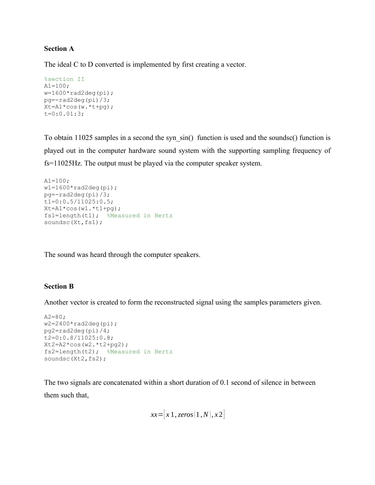
The ideal C to D converted is implemented by first creating a vector.
%section II
A1=100;
w=1600*rad2deg(pi);
pg=-rad2deg(pi)/3;
Xt=A1*cos(w.*t+pg);
t=0:0.01:3;
To obtain 11025 samples in a second the syn_sin() function is used and the soundsc() function is
played out in the computer hardware sound system with the supporting sampling frequency of
fs=11025Hz. The output must be played via the computer speaker system.
A1=100;
w1=1600*rad2deg(pi);
pg=-rad2deg(pi)/3;
t1=0:0.5/11025:0.5;
Xt=A1*cos(w1.*t1+pg);
fs1=length(t1); %Measured in Hertz
soundsc(Xt,fs1);
The sound was heard through the computer speakers.
Section B
Another vector is created to form the reconstructed signal using the samples parameters given.
A2=80;
w2=2400*rad2deg(pi);
pg2=rad2deg(pi)/4;
t2=0:0.8/11025:0.8;
Xt2=A2*cos(w2.*t2+pg2);
fs2=length(t2); %Measured in Hertz
soundsc(Xt2,fs2);
The two signals are concatenated within a short duration of 0.1 second of silence in between
them such that,
xx= [ x 1, zeros ( 1 , N ) , x 2 ]

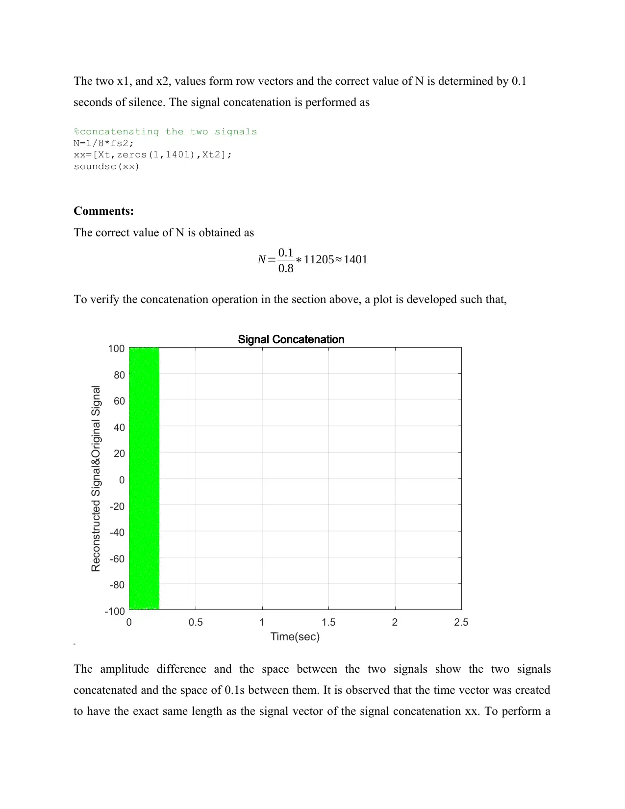
The two x1, and x2, values form row vectors and the correct value of N is determined by 0.1
seconds of silence. The signal concatenation is performed as
%concatenating the two signals
N=1/8*fs2;
xx=[Xt,zeros(1,1401),Xt2];
soundsc(xx)
Comments:
The correct value of N is obtained as
N= 0.1
0.8∗11205≈ 1401
To verify the concatenation operation in the section above, a plot is developed such that,
0 0.5 1 1.5 2 2.5
Time(sec)
-100
-80
-60
-40
-20
0
20
40
60
80
100
Reconstructed Signal&Original Signal
Signal Concatenation
The amplitude difference and the space between the two signals show the two signals
concatenated and the space of 0.1s between them. It is observed that the time vector was created
to have the exact same length as the signal vector of the signal concatenation xx. To perform a

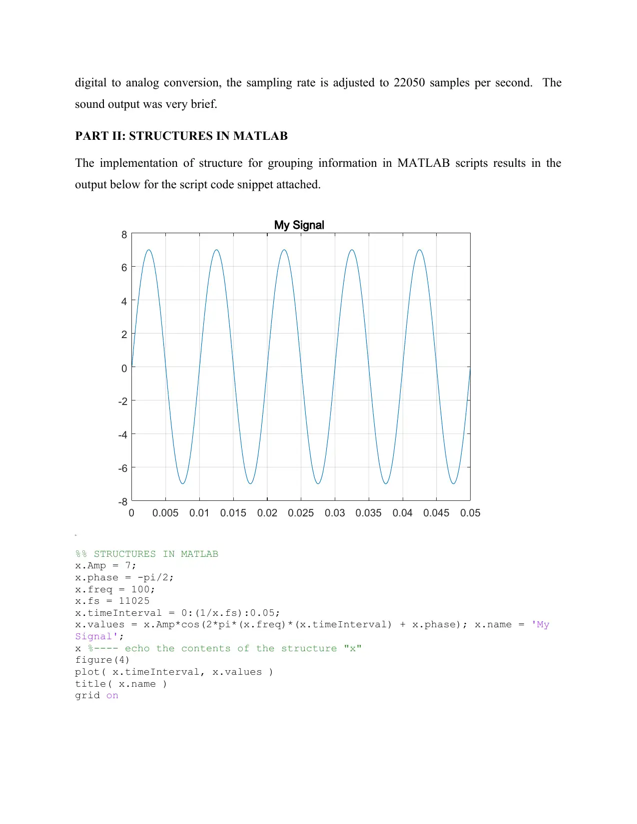
digital to analog conversion, the sampling rate is adjusted to 22050 samples per second. The
sound output was very brief.
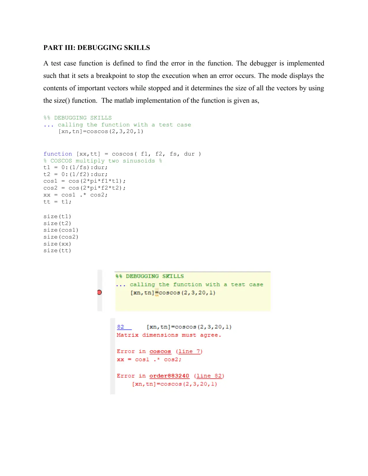
PART II: STRUCTURES IN MATLAB
The implementation of structure for grouping information in MATLAB scripts results in the
output below for the script code snippet attached.
0 0.005 0.01 0.015 0.02 0.025 0.03 0.035 0.04 0.045 0.05
-8
-6
-4
-2
0
2
4
6
8 My Signal
%% STRUCTURES IN MATLAB
x.Amp = 7;
x.phase = -pi/2;
x.freq = 100;
x.fs = 11025
x.timeInterval = 0:(1/x.fs):0.05;
x.values = x.Amp*cos(2*pi*(x.freq)*(x.timeInterval) + x.phase); x.name = 'My
Signal';
x %---- echo the contents of the structure "x"
figure(4)
plot( x.timeInterval, x.values )
title( x.name )
grid on

PART III: DEBUGGING SKILLS
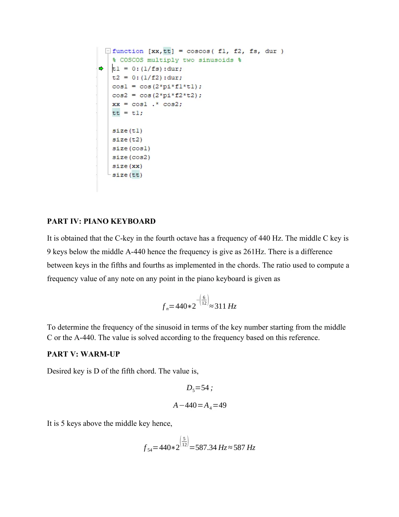
A test case function is defined to find the error in the function. The debugger is implemented
such that it sets a breakpoint to stop the execution when an error occurs. The mode displays the
contents of important vectors while stopped and it determines the size of all the vectors by using
the size() function. The matlab implementation of the function is given as,
%% DEBUGGING SKILLS
... calling the function with a test case
[xn,tn]=coscos(2,3,20,1)
function [xx,tt] = coscos( f1, f2, fs, dur )
% COSCOS multiply two sinusoids %
t1 = 0:(1/fs):dur;
t2 = 0:(1/f2):dur;
cos1 = cos(2*pi*f1*t1);
cos2 = cos(2*pi*f2*t2);
xx = cos1 .* cos2;
tt = t1;
size(t1)
size(t2)
size(cos1)
size(cos2)
size(xx)
size(tt)

PART IV: PIANO KEYBOARD
It is obtained that the C-key in the fourth octave has a frequency of 440 Hz. The middle C key is
9 keys below the middle A-440 hence the frequency is give as 261Hz. There is a difference
between keys in the fifths and fourths as implemented in the chords. The ratio used to compute a
frequency value of any note on any point in the piano keyboard is given as
f n=440∗2−( 6
12 )≈ 311 Hz
To determine the frequency of the sinusoid in terms of the key number starting from the middle
C or the A-440. The value is solved according to the frequency based on this reference.
PART V: WARM-UP
Desired key is D of the fifth chord. The value is,
D5=54 ;
A−440=A4 =49
It is 5 keys above the middle key hence,
f 54=440∗2 ( 5
12 )=587.34 Hz ≈ 587 Hz

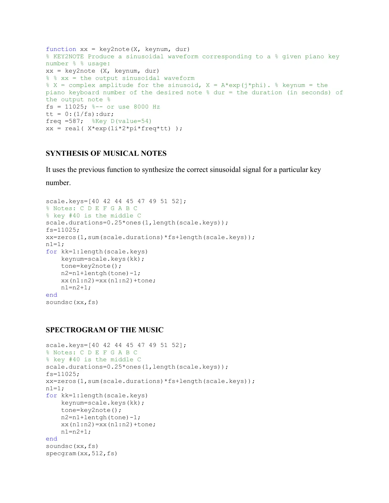
function xx = key2note(X, keynum, dur)
% KEY2NOTE Produce a sinusoidal waveform corresponding to a % given piano key
number % % usage:
xx = key2note (X, keynum, dur)
% % xx = the output sinusoidal waveform
% X = complex amplitude for the sinusoid, X = A*exp(j*phi). % keynum = the
piano keyboard number of the desired note % dur = the duration (in seconds) of
the output note %
fs = 11025; %-- or use 8000 Hz
tt = 0:(1/fs):dur;
freq =587; %Key D(value=54)
xx = real( X*exp(1i*2*pi*freq*tt) );
SYNTHESIS OF MUSICAL NOTES
It uses the previous function to synthesize the correct sinusoidal signal for a particular key
number.
scale.keys=[40 42 44 45 47 49 51 52];
% Notes: C D E F G A B C
% key #40 is the middle C
scale.durations=0.25*ones(1,length(scale.keys));
fs=11025;
xx=zeros(1,sum(scale.durations)*fs+length(scale.keys));
n1=1;
for kk=1:length(scale.keys)
keynum=scale.keys(kk);
tone=key2note();
n2=n1+lentgh(tone)-1;
xx(n1:n2)=xx(n1:n2)+tone;
n1=n2+1;
end
soundsc(xx,fs)
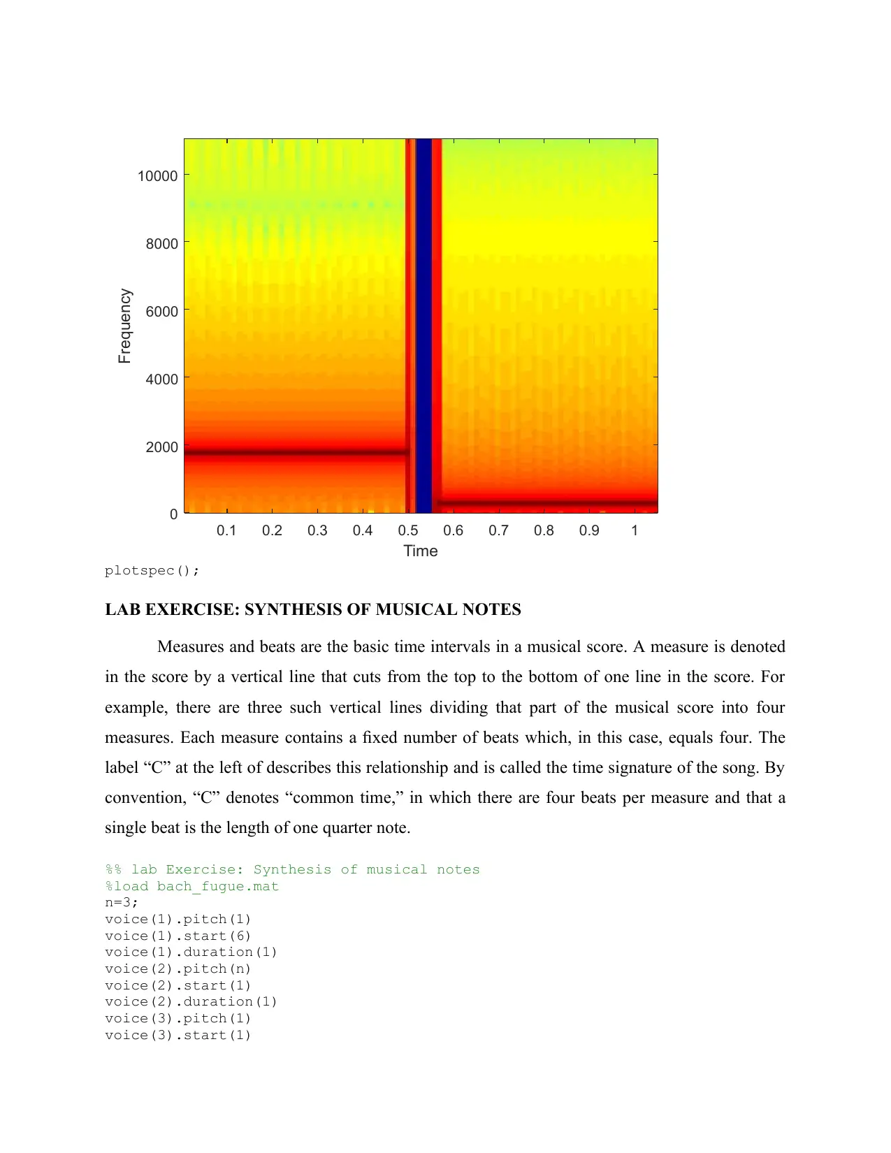
SPECTROGRAM OF THE MUSIC
scale.keys=[40 42 44 45 47 49 51 52];
% Notes: C D E F G A B C
% key #40 is the middle C
scale.durations=0.25*ones(1,length(scale.keys));
fs=11025;
xx=zeros(1,sum(scale.durations)*fs+length(scale.keys));
n1=1;
for kk=1:length(scale.keys)
keynum=scale.keys(kk);
tone=key2note();
n2=n1+lentgh(tone)-1;
xx(n1:n2)=xx(n1:n2)+tone;
n1=n2+1;
end
soundsc(xx,fs)
specgram(xx,512,fs)

0.1 0.2 0.3 0.4 0.5 0.6 0.7 0.8 0.9 1
Time
0
2000
4000
6000
8000
10000
Frequency
plotspec();
LAB EXERCISE: SYNTHESIS OF MUSICAL NOTES
Measures and beats are the basic time intervals in a musical score. A measure is denoted
in the score by a vertical line that cuts from the top to the bottom of one line in the score. For
example, there are three such vertical lines dividing that part of the musical score into four
measures. Each measure contains a fixed number of beats which, in this case, equals four. The
label “C” at the left of describes this relationship and is called the time signature of the song. By
convention, “C” denotes “common time,” in which there are four beats per measure and that a
single beat is the length of one quarter note.
%% lab Exercise: Synthesis of musical notes
%load bach_fugue.mat
n=3;
voice(1).pitch(1)
voice(1).start(6)
voice(1).duration(1)
voice(2).pitch(n)
voice(2).start(1)
voice(2).duration(1)
voice(3).pitch(1)
voice(3).start(1)

voice(3).duration(1)