System Design & Engineering

This document discusses various topics related to system design and engineering. It covers topics such as anticipated impact, risk assessment, manufacturing costs, production capacity, and cash flow analysis. The document provides calculations and explanations for each topic.

SYSTEM DESIGN & ENGINEERING
[Author Name(s), First M. Last, Omit Titles and Degrees]
[Institutional Affiliation(s)]

Question 1
Given that;
We will have to make an assumption for the anticipated impact
High-100k
Medium-75k
Low-50k
Also, assuming that risk is a negative impact on the outcome (Friedman, Hendry & Borning,
2017)
Using the anticipated value method, the following are calculated
C1:340k*60%+100k*10%-50k*30%=199k
C2: 180k*60%+75k*10%-30k*30%=88.5k
C3: 270k*60%+50k*10%-20k*30%=161k
C4: 360k*60%+100k*10%-70k*30%=219k
Since expect risk for C4 is highest, it will be chosen assumption set 2
Assuming the following values for impact
High-10k
Medium-7.5k
Low-5k
C1:190, C2:99.75, C3: 156.5 and C4:196

In this case still, C4 is preferred
Question 2
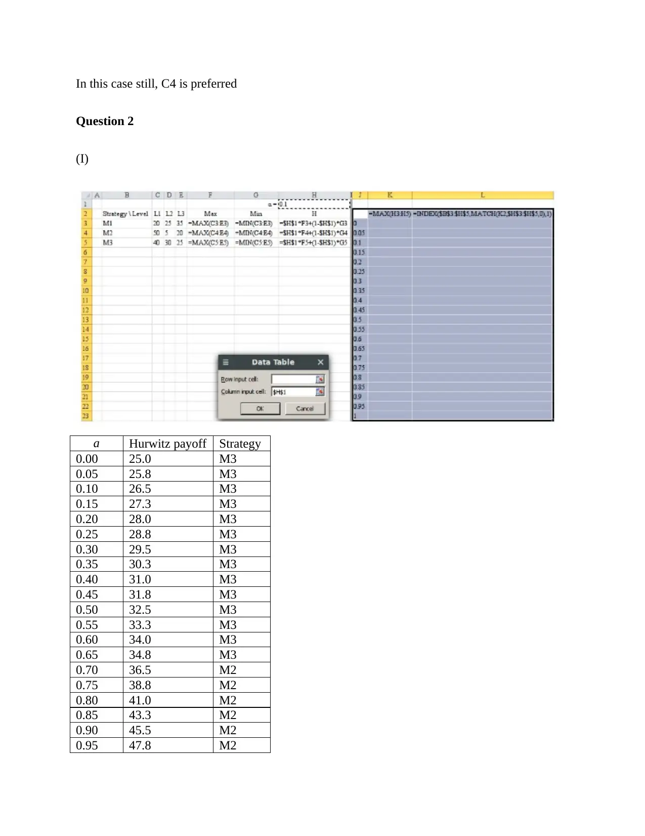
(I)
a Hurwitz payoff Strategy
0.00 25.0 M3
0.05 25.8 M3
0.10 26.5 M3
0.15 27.3 M3
0.20 28.0 M3
0.25 28.8 M3
0.30 29.5 M3
0.35 30.3 M3
0.40 31.0 M3
0.45 31.8 M3
0.50 32.5 M3
0.55 33.3 M3
0.60 34.0 M3
0.65 34.8 M3
0.70 36.5 M2
0.75 38.8 M2
0.80 41.0 M2
0.85 43.3 M2
0.90 45.5 M2
0.95 47.8 M2

1.00 50.0 M2
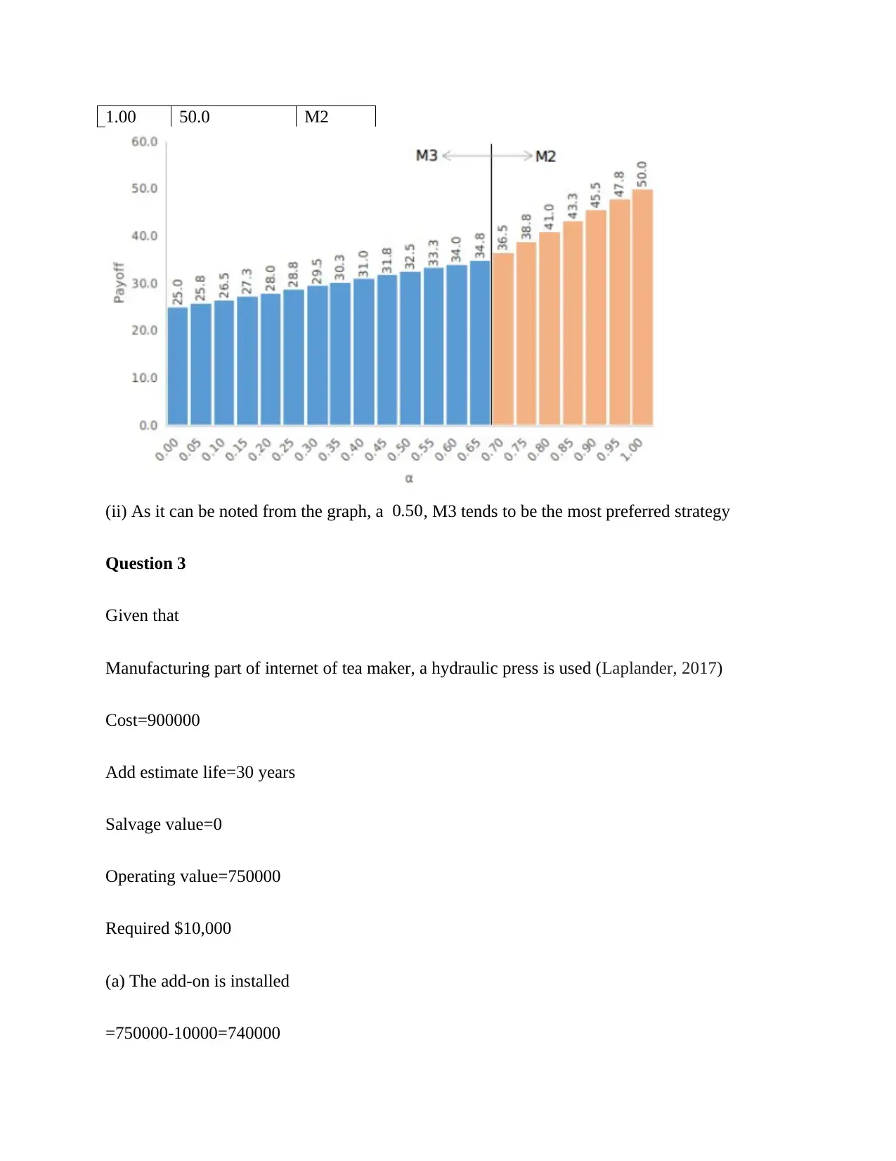
(ii) As it can be noted from the graph, a 0.50, M3 tends to be the most preferred strategy
Question 3
Given that
Manufacturing part of internet of tea maker, a hydraulic press is used (Laplander, 2017)
Cost=900000
Add estimate life=30 years
Salvage value=0
Operating value=750000
Required $10,000
(a) The add-on is installed
=750000-10000=740000

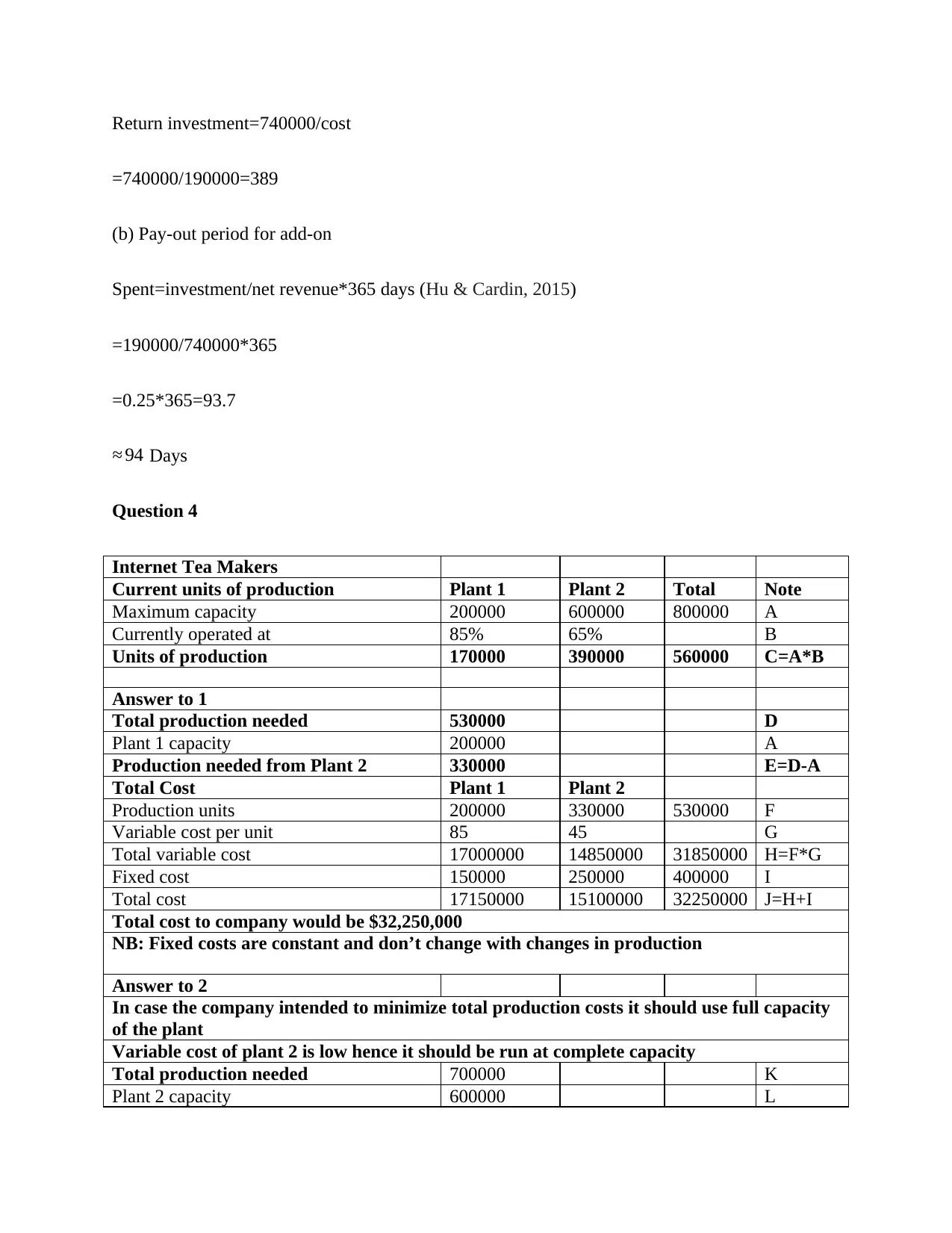
Return investment=740000/cost
=740000/190000=389
(b) Pay-out period for add-on
Spent=investment/net revenue*365 days (Hu & Cardin, 2015)
=190000/740000*365
=0.25*365=93.7
≈ 94 Days
Question 4
Internet Tea Makers
Current units of production Plant 1 Plant 2 Total Note
Maximum capacity 200000 600000 800000 A
Currently operated at 85% 65% B
Units of production 170000 390000 560000 C=A*B
Answer to 1
Total production needed 530000 D
Plant 1 capacity 200000 A
Production needed from Plant 2 330000 E=D-A
Total Cost Plant 1 Plant 2
Production units 200000 330000 530000 F
Variable cost per unit 85 45 G
Total variable cost 17000000 14850000 31850000 H=F*G
Fixed cost 150000 250000 400000 I
Total cost 17150000 15100000 32250000 J=H+I
Total cost to company would be $32,250,000
NB: Fixed costs are constant and don’t change with changes in production
Answer to 2
In case the company intended to minimize total production costs it should use full capacity
of the plant
Variable cost of plant 2 is low hence it should be run at complete capacity
Total production needed 700000 K
Plant 2 capacity 600000 L

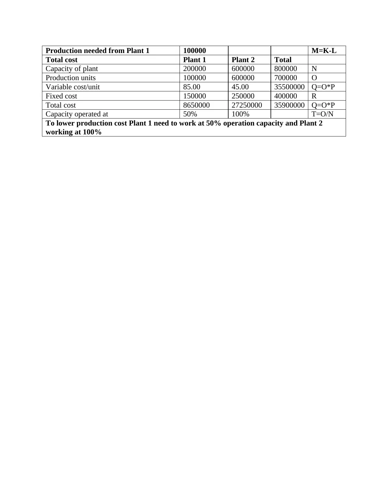
Production needed from Plant 1 100000 M=K-L
Total cost Plant 1 Plant 2 Total
Capacity of plant 200000 600000 800000 N
Production units 100000 600000 700000 O
Variable cost/unit 85.00 45.00 35500000 Q=O*P
Fixed cost 150000 250000 400000 R
Total cost 8650000 27250000 35900000 Q=O*P
Capacity operated at 50% 100% T=O/N
To lower production cost Plant 1 need to work at 50% operation capacity and Plant 2
working at 100%

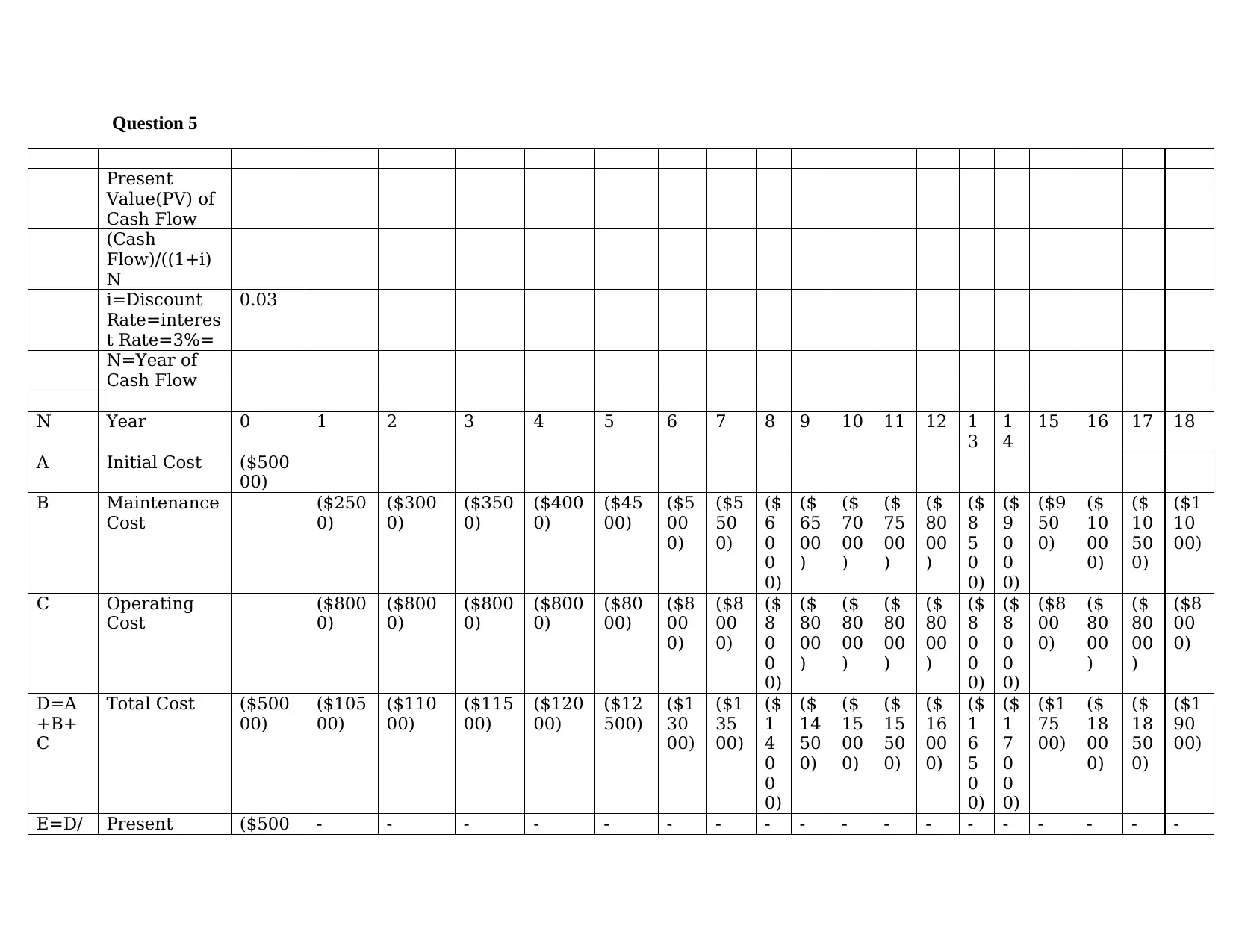
Question 5
Present
Value(PV) of
Cash Flow
(Cash
Flow)/((1+i)
N
i=Discount
Rate=interes
t Rate=3%=
0.03
N=Year of
Cash Flow
N Year 0 1 2 3 4 5 6 7 8 9 10 11 12 1
3
1
4
15 16 17 18
A Initial Cost ($500
00)
B Maintenance
Cost
($250
0)
($300
0)
($350
0)
($400
0)
($45
00)
($5
00
0)
($5
50
0)
($
6
0
0
0)
($
65
00
)
($
70
00
)
($
75
00
)
($
80
00
)
($
8
5
0
0)
($
9
0
0
0)
($9
50
0)
($
10
00
0)
($
10
50
0)
($1
10
00)
C Operating
Cost
($800
0)
($800
0)
($800
0)
($800
0)
($80
00)
($8
00
0)
($8
00
0)
($
8
0
0
0)
($
80
00
)
($
80
00
)
($
80
00
)
($
80
00
)
($
8
0
0
0)
($
8
0
0
0)
($8
00
0)
($
80
00
)
($
80
00
)
($8
00
0)
D=A
+B+
C
Total Cost ($500
00)
($105
00)
($110
00)
($115
00)
($120
00)
($12
500)
($1
30
00)
($1
35
00)
($
1
4
0
0
0)
($
14
50
0)
($
15
00
0)
($
15
50
0)
($
16
00
0)
($
1
6
5
0
0)
($
1
7
0
0
0)
($1
75
00)
($
18
00
0)
($
18
50
0)
($1
90
00)
E=D/ Present ($500 - - - - - - - - - - - - - - - - - -

(1.03
N)
Value of
TotalCost
00) $101
94
$1036
9
$105
24
$106
62
$107
88
$1
08
77
$1
09
77
$
1
1
0
5
2
$1
11
13
$1
11
61
$1
11
98
$1
12
22
$
1
1
2
3
6
$
1
1
2
3
9
$1
12
33
$1
12
17
$1
11
93
$1
11
60
F Cumulative
Present
value of
costs
($601
94)
($705
63)
($810
87)
($917
49)
($10
2531
)
($1
13
41
9)
($1
24
39
5)
($
1
3
5
4
4
7)
($
14
65
60
)
($
15
72
22
)
($
16
89
19
)
($
18
01
41
)
($
1
9
1
3
7
7)
($
2
0
2
6
1
6)
($2
13
84
8)
($
22
50
65
)
($
23
62
58
)
($2
47
41
9)
G Resale Value
(80% of
value of
previous
year)
$400
00
$3200
0
$256
00
$204
80
$163
84
$1
31
07
$1
04
86
$
8
3
8
9
$6
71
1
$5
36
9
$4
29
5
$3
43
6
$
2
7
4
9
$
2
1
9
9
$1
75
9
$1
40
7
$1
12
6
$1
90
1
H=G/
1.03N
Present
Worth of
Resale value
$3883
5
$301
63
$2342
8
$181
96
$141
33
$1
09
77
$8
52
6
$
6
6
2
2
$5
14
3
$3
99
5
$3
10
3
$2
41
0
$
1
8
7
2
$
1
4
5
4
$1
12
9
$8
77
$6
81
$5
29
I=F+
H
Net Present
Worth of
Costs
($213
59)
($404
00)
($576
59)
($735
52)
($88
398)
($1
02
44
2)
($1
15
86
9)
($
1
2
8
8
2
5)
($
14
14
17
)
($
15
37
27
)
($
16
58
16
)
($
17
77
31
)
($
1
8
9
5
0
5)
($
2
0
1
1
6
2)
($2
12
71
9)
($
22
41
88
)
($
23
55
77
)
($2
46
89
0)
J Equated
Uniform
AnnualCost
$220
00
$2111
3
$203
84
$197
88
$189
10
$1
85
98
$1
83
52
$
1
8
1
6
3
$1
80
21
$1
79
21
$1
78
55
$1
79
21
$
1
7
8
5
5
$
1
7
8
0
8
$1
78
19
$1
78
48
$1
78
93
$1
79
51

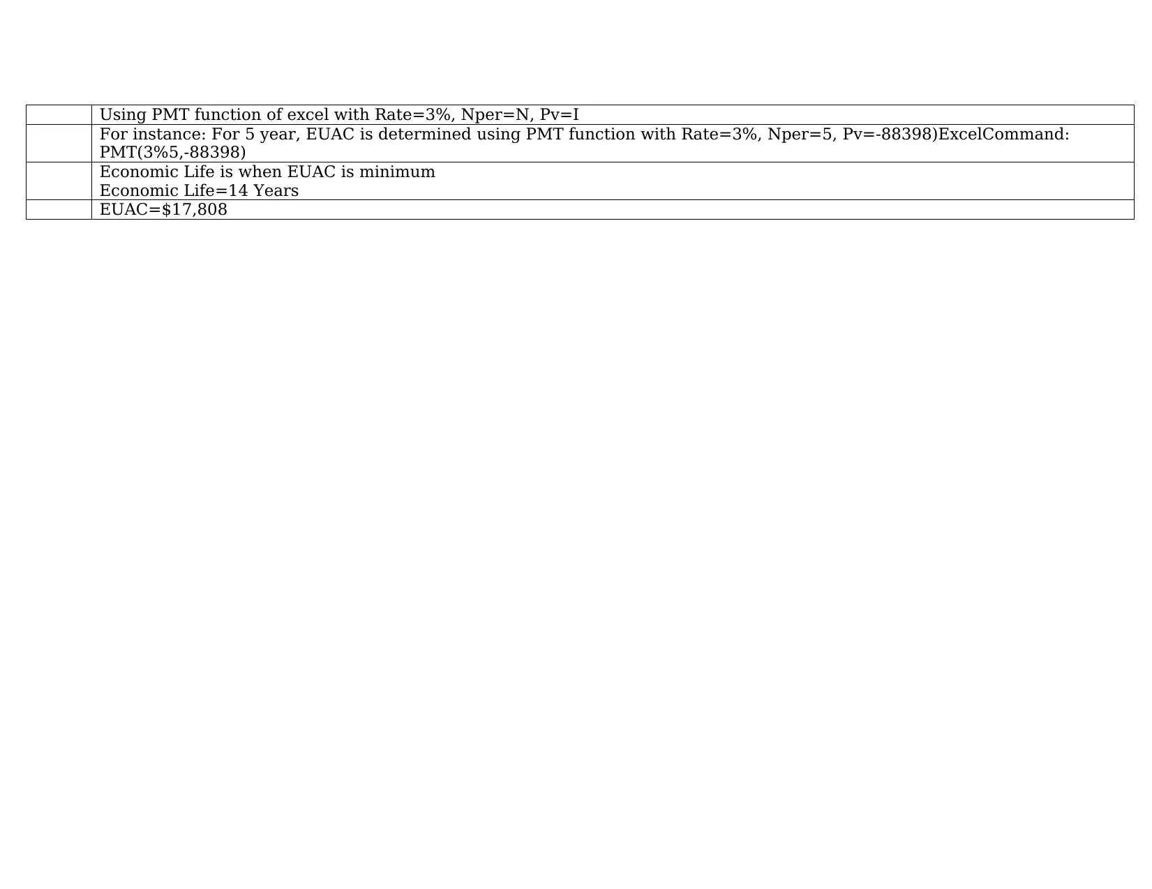
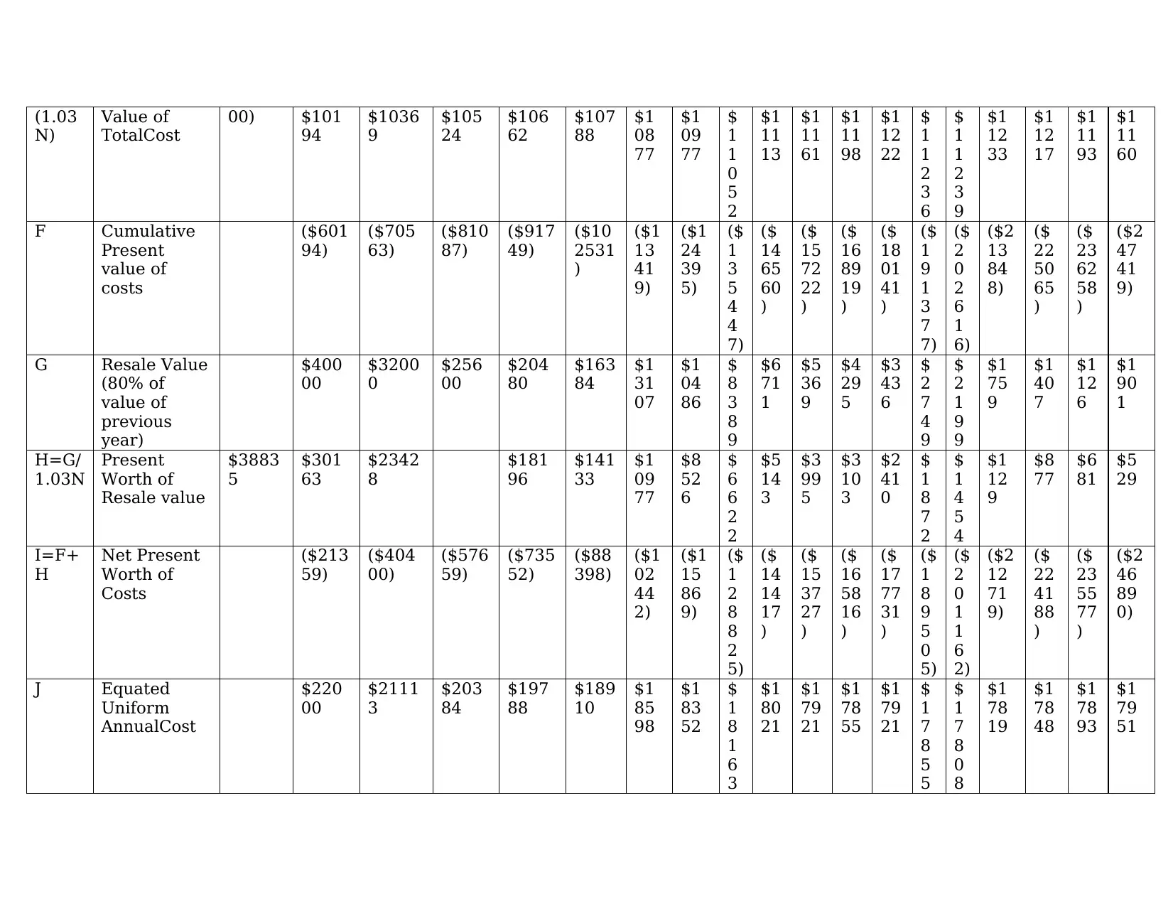
Using PMT function of excel with Rate=3%, Nper=N, Pv=I
For instance: For 5 year, EUAC is determined using PMT function with Rate=3%, Nper=5, Pv=-88398)ExcelCommand:
PMT(3%5,-88398)
Economic Life is when EUAC is minimum
Economic Life=14 Years
EUAC=$17,808

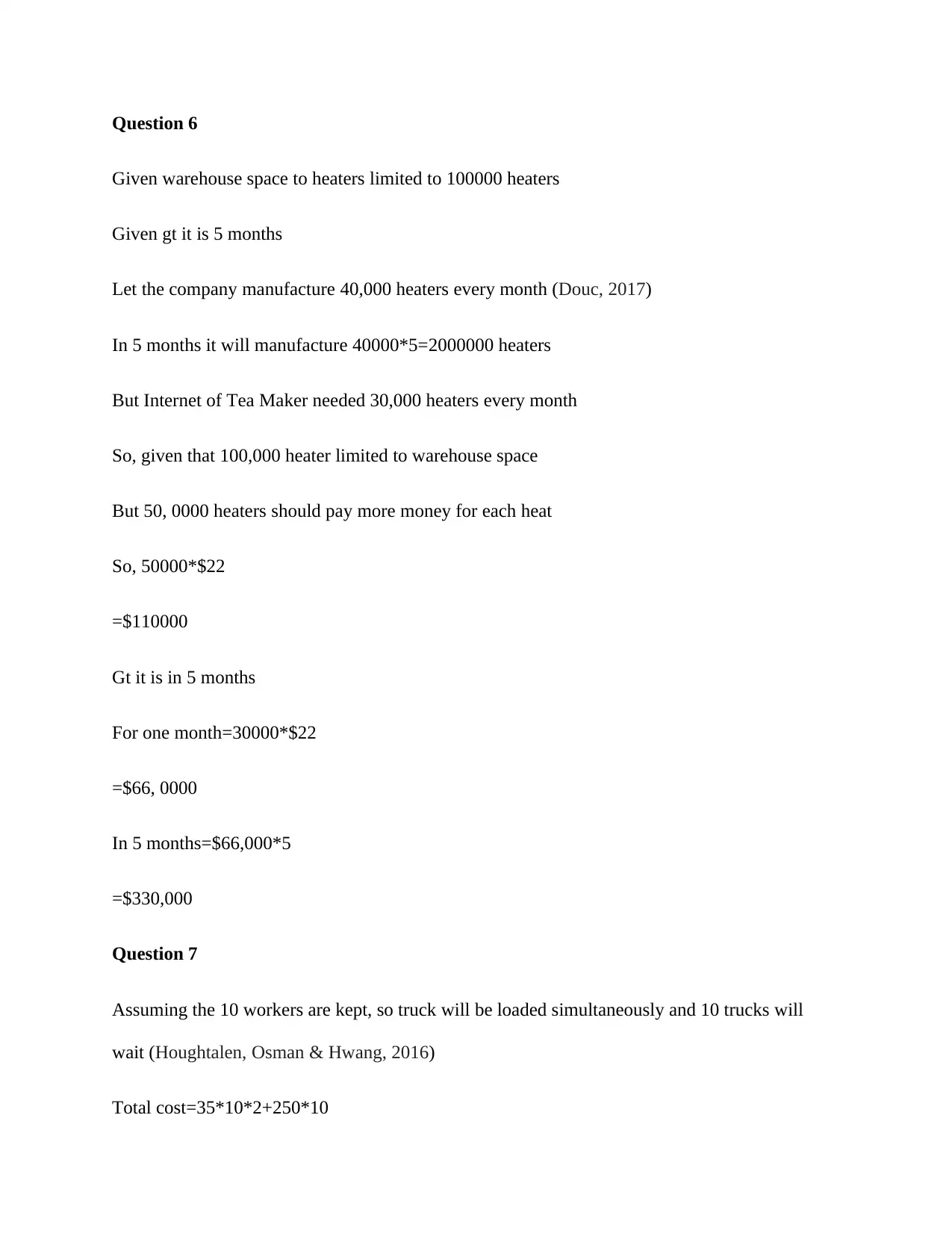
Question 6
Given warehouse space to heaters limited to 100000 heaters
Given gt it is 5 months
Let the company manufacture 40,000 heaters every month (Douc, 2017)
In 5 months it will manufacture 40000*5=2000000 heaters
But Internet of Tea Maker needed 30,000 heaters every month
So, given that 100,000 heater limited to warehouse space
But 50, 0000 heaters should pay more money for each heat
So, 50000*$22
=$110000
Gt it is in 5 months
For one month=30000*$22
=$66, 0000
In 5 months=$66,000*5
=$330,000
Question 7
Assuming the 10 workers are kept, so truck will be loaded simultaneously and 10 trucks will
wait (Houghtalen, Osman & Hwang, 2016)
Total cost=35*10*2+250*10

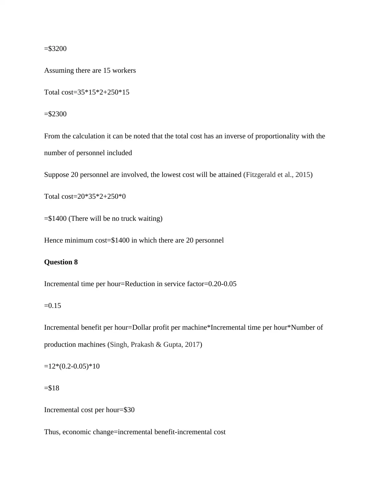
=$3200
Assuming there are 15 workers
Total cost=35*15*2+250*15
=$2300
From the calculation it can be noted that the total cost has an inverse of proportionality with the
number of personnel included
Suppose 20 personnel are involved, the lowest cost will be attained (Fitzgerald et al., 2015)
Total cost=20*35*2+250*0
=$1400 (There will be no truck waiting)
Hence minimum cost=$1400 in which there are 20 personnel
Question 8
Incremental time per hour=Reduction in service factor=0.20-0.05
=0.15
Incremental benefit per hour=Dollar profit per machine*Incremental time per hour*Number of
production machines (Singh, Prakash & Gupta, 2017)
=12*(0.2-0.05)*10
=$18
Incremental cost per hour=$30
Thus, economic change=incremental benefit-incremental cost

=18-30=-$12
Question 9
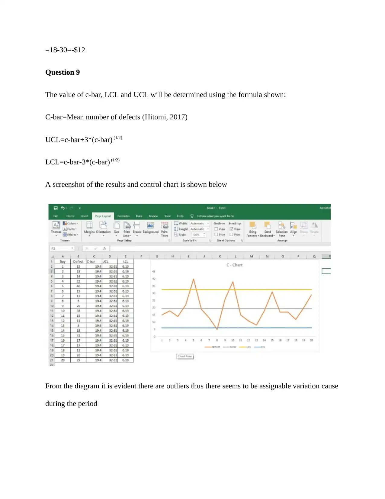
The value of c-bar, LCL and UCL will be determined using the formula shown:
C-bar=Mean number of defects (Hitomi, 2017)
UCL=c-bar+3*(c-bar) (1/2)
LCL=c-bar-3*(c-bar) (1/2)
A screenshot of the results and control chart is shown below
From the diagram it is evident there are outliers thus there seems to be assignable variation cause
during the period

Question 10
The most critical path is the path marked red
The path A-B-E-G tends to be the most critical path and need 29 weeks for completion of task

References
Dbouk, T. (2017). A review about the engineering design of optimal heat transfer systems using
topology optimization. Applied Thermal Engineering, 112, 841-854
Fitzgerald, J., Gamble, C., Larsen, P. G., Pierce, K., & Woodcock, J. (2015, May). Cyber-
physical systems design: formal foundations, methods and integrated tool chains. In 2015
IEEE/ACM 3rd FME Workshop on Formal Methods in Software Engineering (pp. 40-
46). IEEE
Friedman, B., Hendry, D. G., & Borning, A. (2017). A survey of value sensitive design
methods. Foundations and Trends® in Human–Computer Interaction, 11(2), 63-125
Harrison, R., Vera, D., & Ahmad, B. (2016). Engineering methods and tools for cyber–physical
automation systems. Proceedings of the IEEE, 104(5), 973-985
Hitomi, K. (2017). Manufacturing systems engineering: A unified approach to manufacturing
technology, production management and industrial economics. Routledge
Houghtalen, R. J., Osman, A., & Hwang, N. H. (2016). Fundamentals of hydraulic engineering
systems. New York: Prentice Hall
Hu, J., & Cardin, M. A. (2015). Generating flexibility in the design of engineering systems to
enable better sustainability and lifecycle performance. Research in Engineering
Design, 26(2), 121-143
Laplante, P. A. (2017). Requirements engineering for software and systems. Auerbach
Publications

Singh, N., Prakash, J., & Gupta, R. K. (2017). Design and engineering of high-performance
photocatalytic systems based on metal oxide–graphene–noble metal
nanocomposites. Molecular Systems Design & Engineering, 2(4), 422-439