Simulation of a Harmonic Equation with Built-in Tests

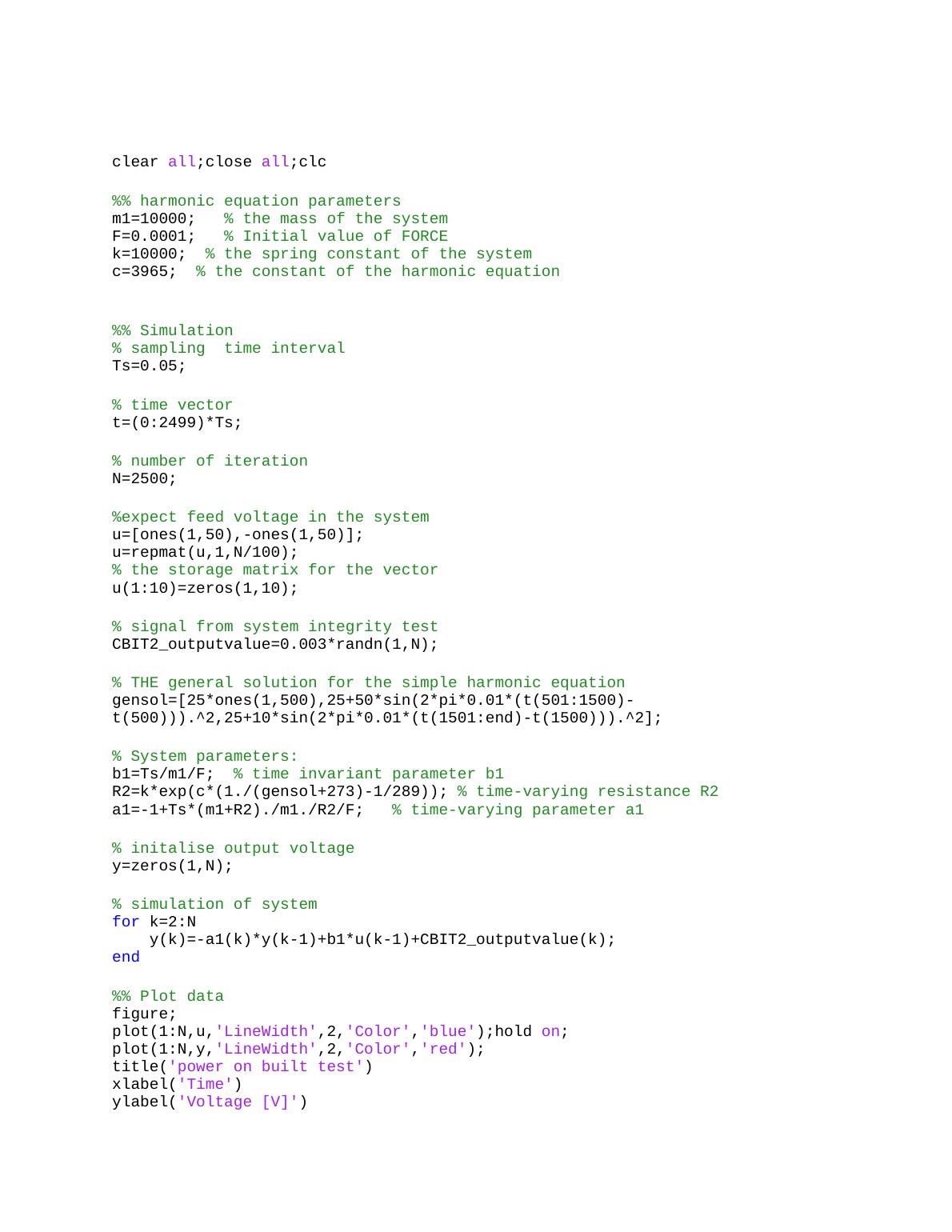
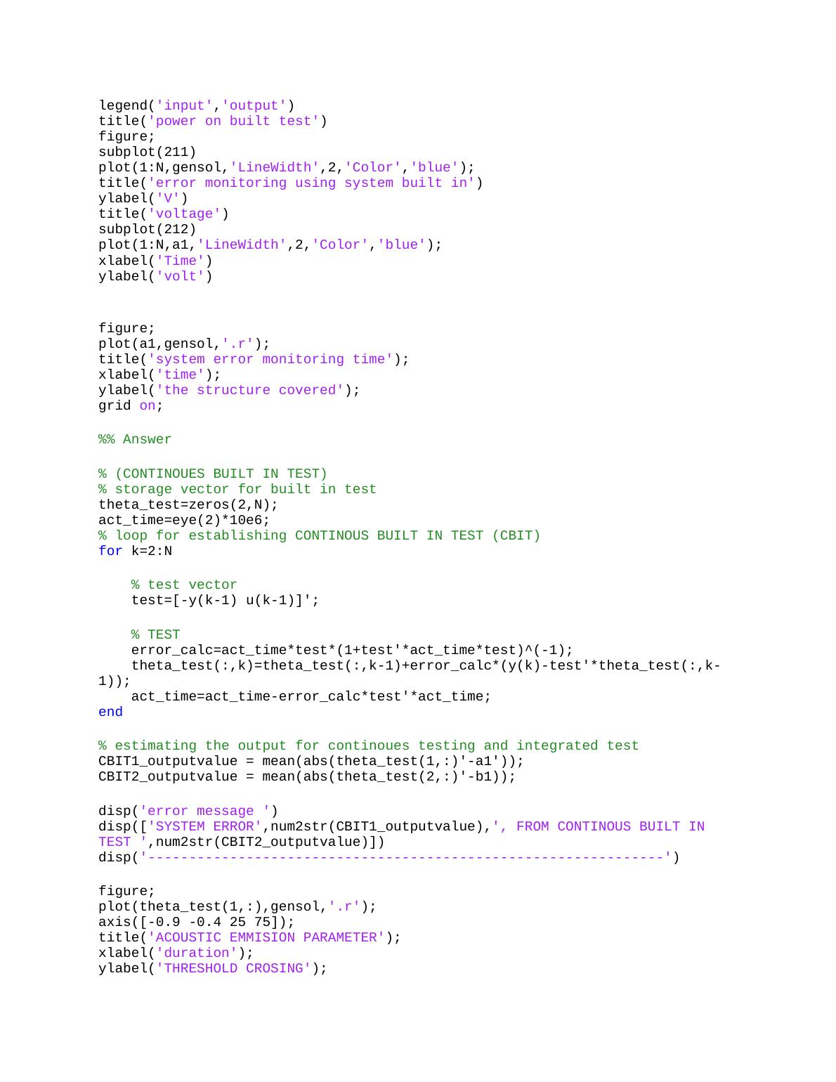
This MATLAB code simulates a harmonic equation with built-in tests for error monitoring and system integrity testing. The simulation includes continuous built-in tests, system integrated tests, and initiated built-in tests. The code also includes plots for error monitoring and system failure analysis.

clear all;close all;clc
%% harmonic equation parameters
m1=10000; % the mass of the system
F=0.0001; % Initial value of FORCE
k=10000; % the spring constant of the system
c=3965; % the constant of the harmonic equation
%% Simulation
% sampling time interval
Ts=0.05;
% time vector
t=(0:2499)*Ts;
% number of iteration
N=2500;
%expect feed voltage in the system
u=[ones(1,50),-ones(1,50)];
u=repmat(u,1,N/100);
% the storage matrix for the vector
u(1:10)=zeros(1,10);
% signal from system integrity test
CBIT2_outputvalue=0.003*randn(1,N);
% THE general solution for the simple harmonic equation
gensol=[25*ones(1,500),25+50*sin(2*pi*0.01*(t(501:1500)-
t(500))).^2,25+10*sin(2*pi*0.01*(t(1501:end)-t(1500))).^2];
% System parameters:
b1=Ts/m1/F; % time invariant parameter b1
R2=k*exp(c*(1./(gensol+273)-1/289)); % time-varying resistance R2
a1=-1+Ts*(m1+R2)./m1./R2/F; % time-varying parameter a1
% initalise output voltage
y=zeros(1,N);
% simulation of system
for k=2:N
y(k)=-a1(k)*y(k-1)+b1*u(k-1)+CBIT2_outputvalue(k);
end
%% Plot data
figure;
plot(1:N,u,'LineWidth',2,'Color','blue');hold on;
plot(1:N,y,'LineWidth',2,'Color','red');
title('power on built test')
xlabel('Time')
ylabel('Voltage [V]')

legend('input','output')
title('power on built test')
figure;
subplot(211)
plot(1:N,gensol,'LineWidth',2,'Color','blue');
title('error monitoring using system built in')
ylabel('V')
title('voltage')
subplot(212)
plot(1:N,a1,'LineWidth',2,'Color','blue');
xlabel('Time')
ylabel('volt')
figure;
plot(a1,gensol,'.r');
title('system error monitoring time');
xlabel('time');
ylabel('the structure covered');
grid on;
%% Answer
% (CONTINOUES BUILT IN TEST)
% storage vector for built in test
theta_test=zeros(2,N);
act_time=eye(2)*10e6;
% loop for establishing CONTINOUS BUILT IN TEST (CBIT)
for k=2:N
% test vector
test=[-y(k-1) u(k-1)]';
% TEST
error_calc=act_time*test*(1+test'*act_time*test)^(-1);
theta_test(:,k)=theta_test(:,k-1)+error_calc*(y(k)-test'*theta_test(:,k-
1));
act_time=act_time-error_calc*test'*act_time;
end
% estimating the output for continoues testing and integrated test
CBIT1_outputvalue = mean(abs(theta_test(1,:)'-a1'));
CBIT2_outputvalue = mean(abs(theta_test(2,:)'-b1));
disp('error message ')
disp(['SYSTEM ERROR',num2str(CBIT1_outputvalue),', FROM CONTINOUS BUILT IN
TEST ',num2str(CBIT2_outputvalue)])
disp('---------------------------------------------------------------')
figure;
plot(theta_test(1,:),gensol,'.r');
axis([-0.9 -0.4 25 75]);
title('ACOUSTIC EMMISION PARAMETER');
xlabel('duration');
ylabel('THRESHOLD CROSING');

grid on;
% SYSTEN INTEGRATED TEST
%STORAGE matrix
theta_SInT=zeros(2,N);
act_time=eye(2)*10e6;
lam = 0.97;
% loop for establishing System Integrity Test (SInT)
for k=2:N
% test vector
test=[-y(k-1) u(k-1)]';
% SInT test
error_calc=act_time*test*(lam+test'*act_time*test)^(-1);
theta_SInT(:,k)=theta_SInT(:,k-1)+error_calc*(y(k)-test'*theta_SInT(:,k-
1));
act_time=(1/lam)*(act_time-error_calc*test'*act_time);
end
SInT1_outputvalue = mean(abs(theta_SInT(1,:)'-a1'));
SInT2_outputvalue = mean(abs(theta_SInT(2,:)'-b1));
disp('ERROR MESSAGE ')
disp(['SYSTEM ERROR ',num2str(SInT1_outputvalue),', FROM SYSTEM INTEGRITING
TEST ',num2str(SInT2_outputvalue)])
disp('---------------------------------------------------------------')
figure;
plot(theta_SInT(1,:),gensol,'.r');
axis([-0.9 -0.4 25 75]);
title('ACOUSTIC EMMISION PARAMETER2');
xlabel('duration');
ylabel('THRESHOLD CROSING');
grid on;
% initiated built in test
theta_init=zeros(2,N);
act_time=eye(2)*10e6;
lam = 0.97;
for k=2:N
% IBIT vector
test=[-y(k-1) u(k-1)]';
% step prediction
act_time=act_time+[1 0; 0 0];
% IBIT
error_calc=act_time*test*(lam+test'*act_time*test)^(-1);
theta_init(:,k)=theta_init(:,k-1)+error_calc*(y(k)-test'*theta_init(:,k-
1));

act_time=act_time-error_calc*test'*act_time;
end
IBIT1_outputvalue = mean(abs(theta_init(1,:)'-a1'));
IBIT2_outputvalue = mean(abs(theta_init(2,:)'-b1));
disp('IBT ERROR')
disp(['SYSTEM FAILURE ',num2str(IBIT1_outputvalue),', FROM IBIT
',num2str(IBIT2_outputvalue)])
disp('---------------------------------------------------------------')
figure;
plot(theta_init(1,:),gensol,'.r');
axis([-0.9 -0.4 25 75]);
title('(IBIT) Scatter plot for parameter ');
xlabel('VOLT');
ylabel('Time');
grid on;