Introduction to Data Science
VerifiedAdded on 2022/12/29
|11
|3150
|22
AI Summary
This document provides an introduction to data science and covers topics such as data setup, exploratory data analysis, one-variable analysis, advanced analysis techniques like clustering and linear regression, and more. The dataset used for analysis is the Australian Road Death Database from 2010 to 2018. The document includes graphs and explanations to help visualize and understand the analysis.
Contribute Materials
Your contribution can guide someone’s learning journey. Share your
documents today.
Table of Contents
Executive summary.....................................................................................................................................1
Introduction.................................................................................................................................................2
Data setup...................................................................................................................................................2
Exploratory data analysis.............................................................................................................................2
One-variable analysis...............................................................................................................................2
Advanced analysis.......................................................................................................................................6
Clustering................................................................................................................................................6
Brief explanation of k-means and clustering.......................................................................................6
Clustering analysis...................................................................................................................................7
Linear regression.....................................................................................................................................8
Brief definition of linear regression.....................................................................................................8
Conclusion.................................................................................................................................................10
Reflections.................................................................................................................................................10
References.................................................................................................................................................11
Introduction to data science
Executive summary
The dataset is first processed then used for analysis. The dataset from
(https://data.gov.au/data/dataset/australian-road-deaths-database ) or blackboard will be
setup and pre-processed. The following analysis will be performed; one-variable analysis and
two-variable analysis. A graph will be provided for each analysis to enable better visualization of
the mentioned analysis. Advance analysis will also be carried out and it includes clustering and
linear regression. Clustering and k-means will be explained briefly thereafter clustering analysis
to group years will be performed. Linear regression is explained briefly and also linear
regression analysis is done and the model plotted.
Secure Best Marks with AI Grader
Need help grading? Try our AI Grader for instant feedback on your assignments.
Introduction
The data analysis research report has been carried out to find out the patterns in the study of
the Australian road transport crash fatalities from 2010 to 2018. There are no specific
objectives to be achieved from this research report analysis however if anything is found to be
worth studying or significant then it will be thoroughly analyzed so as to help other researchers,
government agencies and business representatives. The given dataset about the Australian
road death fatalities will be critically analyzed. The dataset is obtained from the blackboard or
the website (https://data.gov.au/data/dataset/australian-road-deaths-database ). The
Australian Road Death Database (ARDD) contains basic demographic and crash details of people
who died in Australia road crash. A road crash or death means that a person dies within 30 days
due to injuries obtained from the crash. From the given dataset a value of -9 represents missing
or unknown value. The dataset consist of 20 variables or columns and some attributes are
numeric while others are string or categorical. Moreover the Australian road transport crash
fatalities from 2010 to 2018 contain 11,133 rows.
Data setup
Before the dataset is loaded into R programming, the raw “BITREARDDFatalities.csv” file is pre-
processed. Many rows are left blank or estimated with a value of -9 to represent unrecorded or
missing data. When these values of -9 are changed using the excel replace function then cutting
these rows out will be easier in R. Now the subset of the dataset “BITREARDDFatalities.csv” is
loaded into the workspace. There is a command getwd() in R which is used to find the location
of the workspace.
> #location of workspace
> getwd()
[1] "C:/Users/JARO/Documents"
The location of the workspace is confirmed “road transport 3.xlsx” and it is placed in the
workspace location. Now that the raw data is an excel workbook file or .xlsx which is not a text
file, the built in function in R called xlsx reader can be used to read the file information.
Exploratory data analysis
One-variable analysis
> #histogram one-variable analysis
> speed=road_transport_3$`Speed Limit`
> hist(speed)
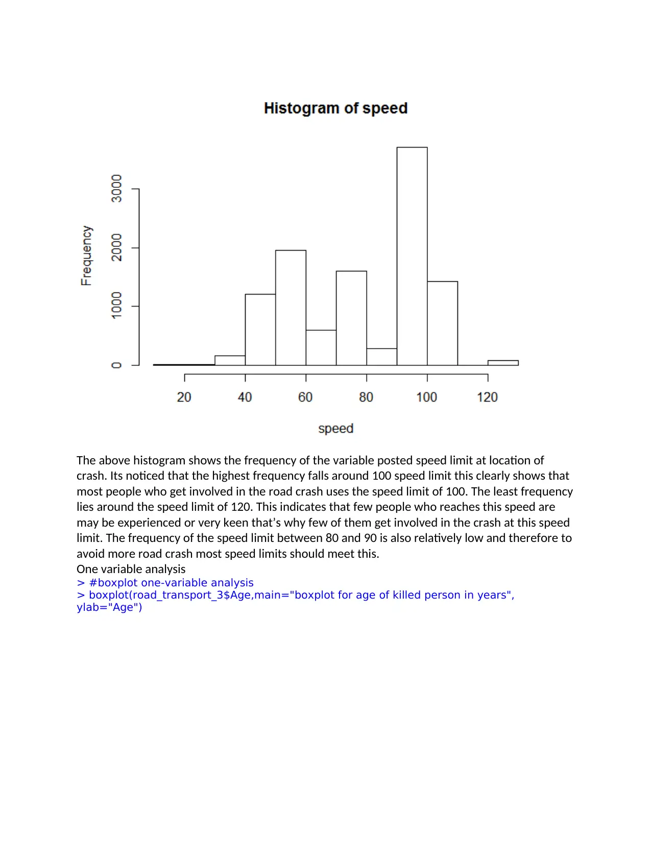
The above histogram shows the frequency of the variable posted speed limit at location of
crash. Its noticed that the highest frequency falls around 100 speed limit this clearly shows that
most people who get involved in the road crash uses the speed limit of 100. The least frequency
lies around the speed limit of 120. This indicates that few people who reaches this speed are
may be experienced or very keen that’s why few of them get involved in the crash at this speed
limit. The frequency of the speed limit between 80 and 90 is also relatively low and therefore to
avoid more road crash most speed limits should meet this.
One variable analysis
> #boxplot one-variable analysis
> boxplot(road_transport_3$Age,main="boxplot for age of killed person in years",
ylab="Age")
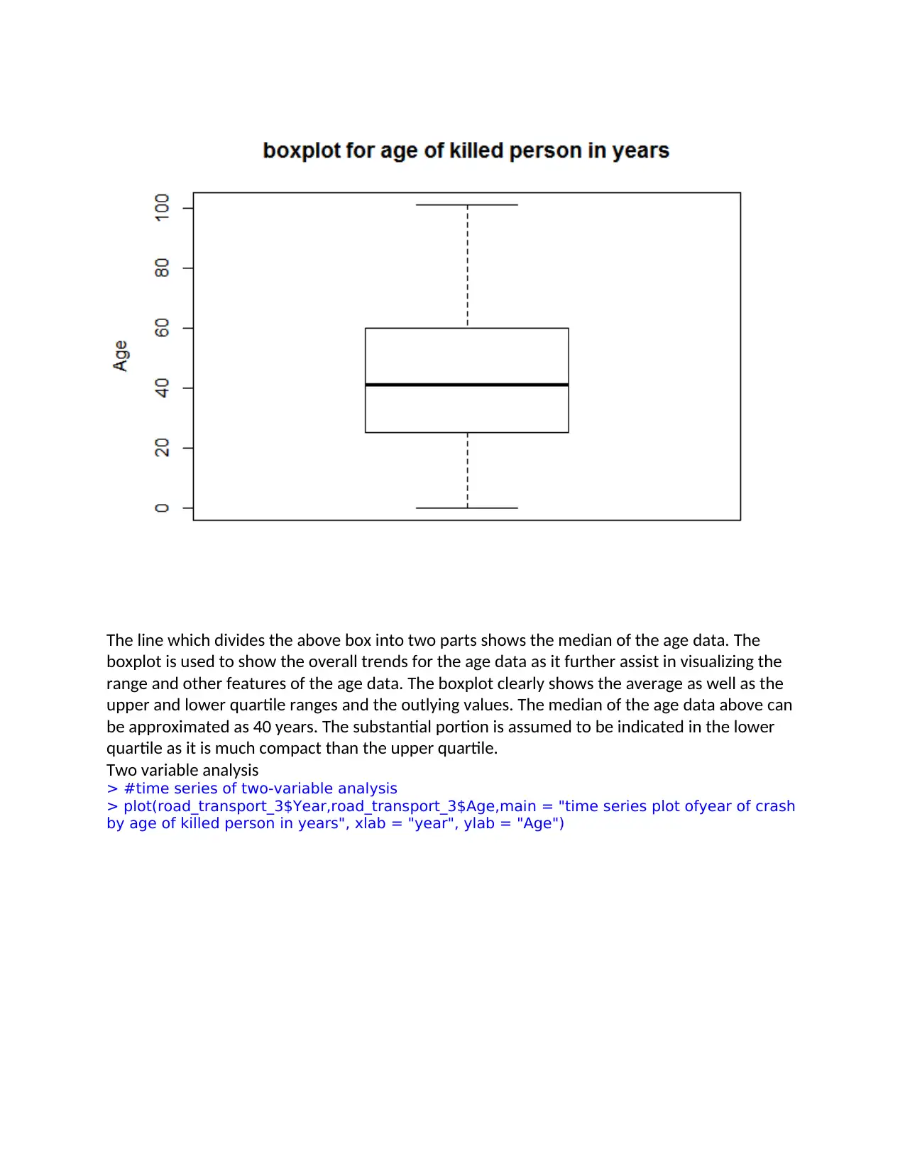
The line which divides the above box into two parts shows the median of the age data. The
boxplot is used to show the overall trends for the age data as it further assist in visualizing the
range and other features of the age data. The boxplot clearly shows the average as well as the
upper and lower quartile ranges and the outlying values. The median of the age data above can
be approximated as 40 years. The substantial portion is assumed to be indicated in the lower
quartile as it is much compact than the upper quartile.
Two variable analysis
> #time series of two-variable analysis
> plot(road_transport_3$Year,road_transport_3$Age,main = "time series plot ofyear of crash
by age of killed person in years", xlab = "year", ylab = "Age")
Secure Best Marks with AI Grader
Need help grading? Try our AI Grader for instant feedback on your assignments.
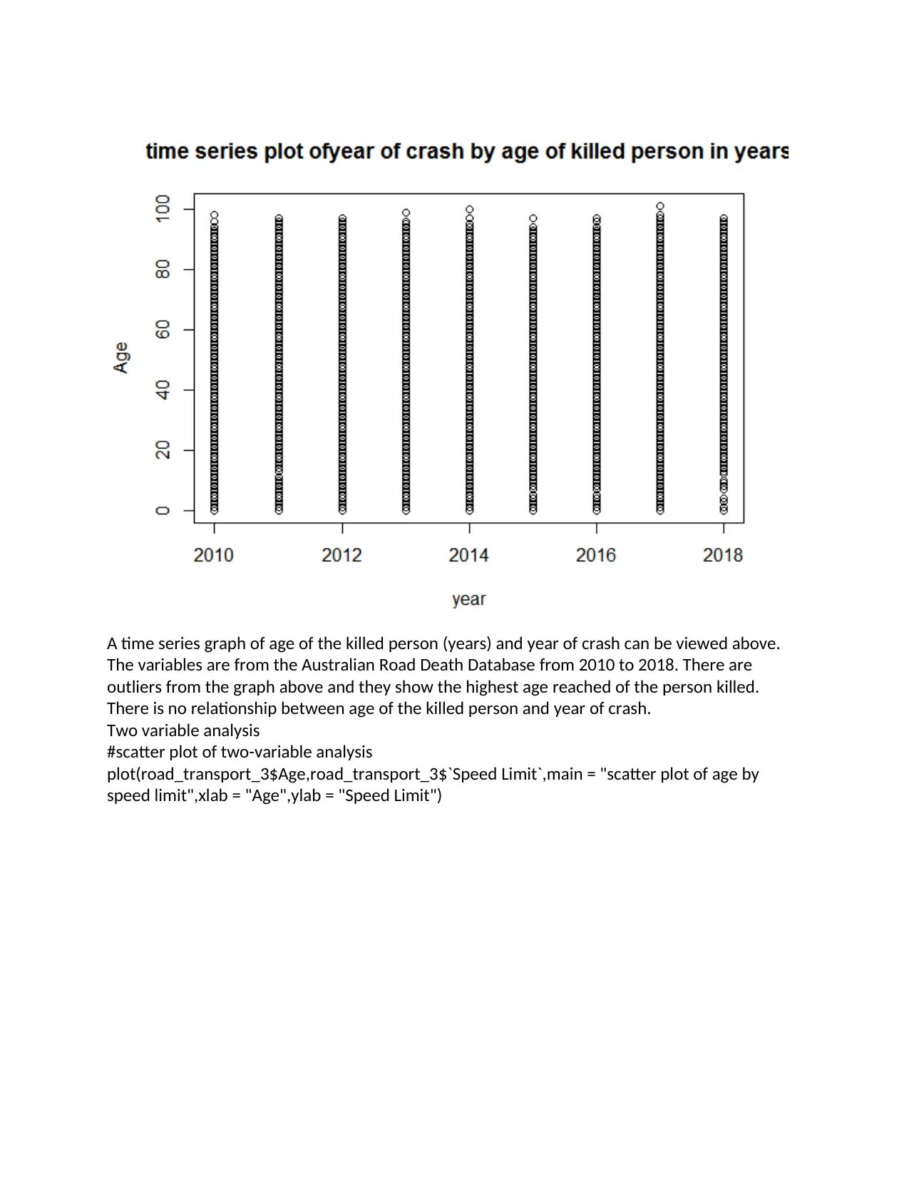
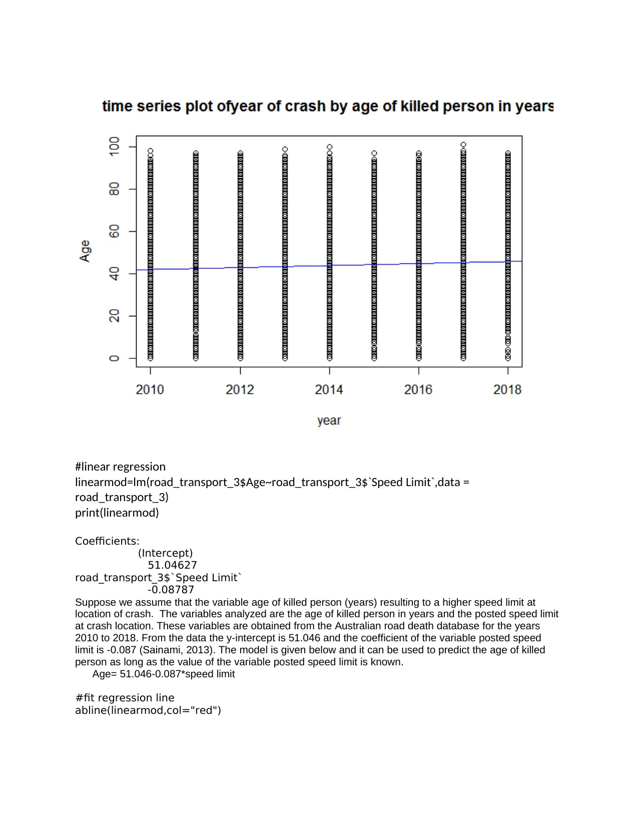
A time series graph of age of the killed person (years) and year of crash can be viewed above.
The variables are from the Australian Road Death Database from 2010 to 2018. There are
outliers from the graph above and they show the highest age reached of the person killed.
There is no relationship between age of the killed person and year of crash.
Two variable analysis
#scatter plot of two-variable analysis
plot(road_transport_3$Age,road_transport_3$`Speed Limit`,main = "scatter plot of age by
speed limit",xlab = "Age",ylab = "Speed Limit")
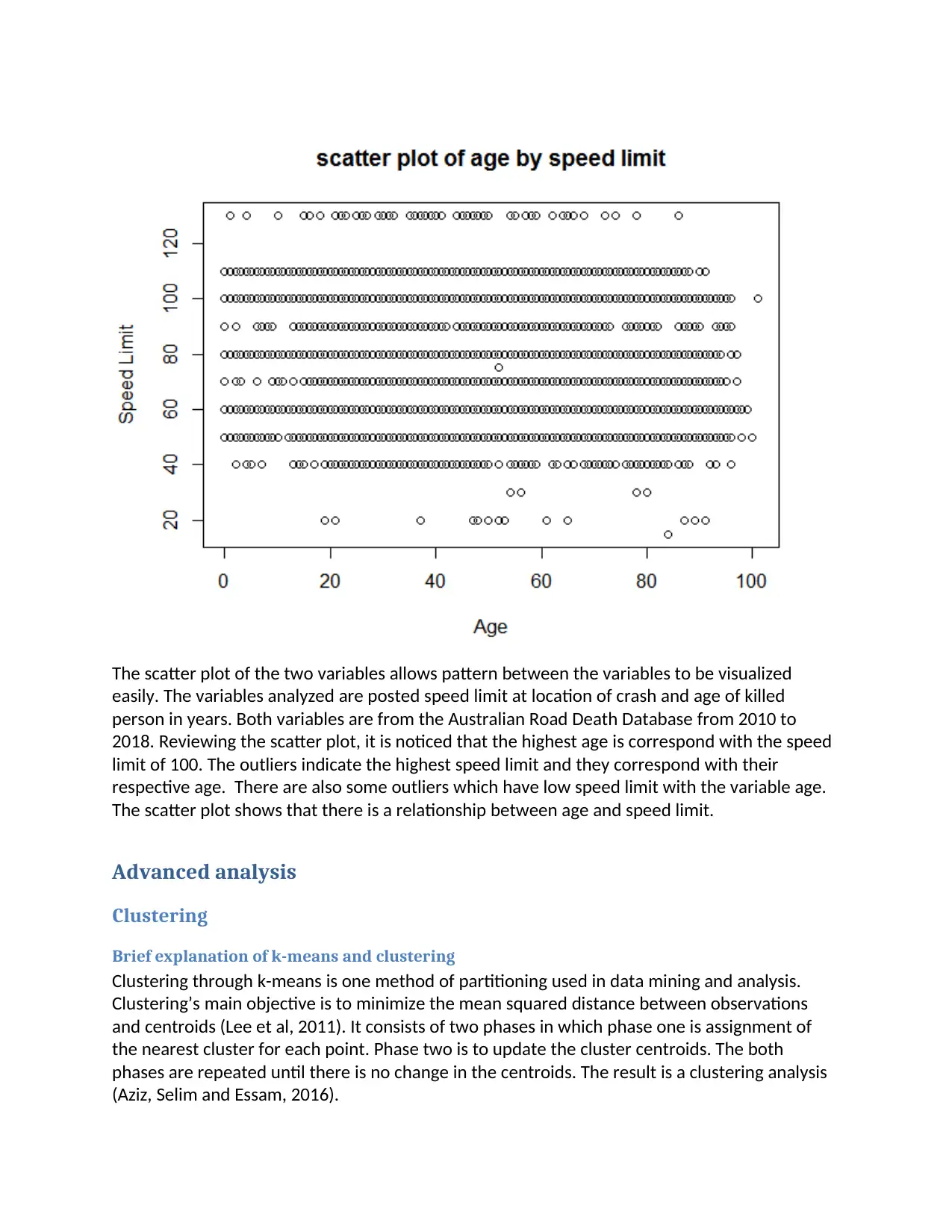
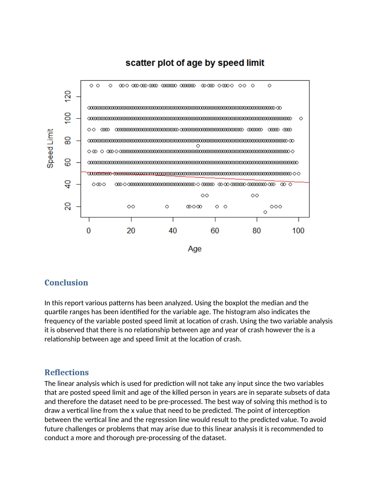
The scatter plot of the two variables allows pattern between the variables to be visualized
easily. The variables analyzed are posted speed limit at location of crash and age of killed
person in years. Both variables are from the Australian Road Death Database from 2010 to
2018. Reviewing the scatter plot, it is noticed that the highest age is correspond with the speed
limit of 100. The outliers indicate the highest speed limit and they correspond with their
respective age. There are also some outliers which have low speed limit with the variable age.
The scatter plot shows that there is a relationship between age and speed limit.
Advanced analysis
Clustering
Brief explanation of k-means and clustering
Clustering through k-means is one method of partitioning used in data mining and analysis.
Clustering’s main objective is to minimize the mean squared distance between observations
and centroids (Lee et al, 2011). It consists of two phases in which phase one is assignment of
the nearest cluster for each point. Phase two is to update the cluster centroids. The both
phases are repeated until there is no change in the centroids. The result is a clustering analysis
(Aziz, Selim and Essam, 2016).
Clustering analysis
#Clustering
road_transport_2_stand=road_transport_2
road_transport_2_stand$Year=NULL
road_transport_2_stand=na.omit(road_transport_2_stand)
road_transport_2_stand=scale(road_transport_2_stand)
fit=kmeans(road_transport_2_stand,4)
fit
fit$cluster
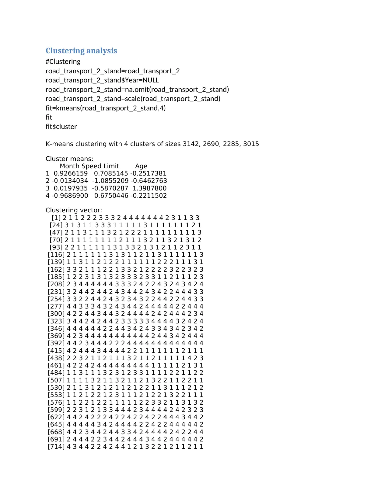
K-means clustering with 4 clusters of sizes 3142, 2690, 2285, 3015
Cluster means:
Month Speed Limit Age
1 0.9266159 0.7085145 -0.2517381
2 -0.0134034 -1.0855209 -0.6462763
3 0.0197935 -0.5870287 1.3987800
4 -0.9686900 0.6750446 -0.2211502
Clustering vector:
[1] 2 1 1 2 2 2 3 3 3 2 4 4 4 4 4 4 4 2 3 1 1 3 3
[24] 3 1 3 1 1 3 3 3 1 1 1 1 1 3 1 1 1 1 1 1 1 2 1
[47] 2 1 1 3 1 1 1 3 2 1 2 2 2 1 1 1 1 1 1 1 1 1 3
[70] 2 1 1 1 1 1 1 1 1 2 1 1 1 3 2 1 1 3 2 1 3 1 2
[93] 2 2 1 1 1 1 1 1 3 1 3 3 2 1 3 1 2 1 1 2 3 1 1
[116] 2 1 1 1 1 1 1 3 1 3 1 1 2 1 1 3 1 1 1 1 1 1 3
[139] 1 1 3 1 1 2 1 2 2 1 1 1 1 1 1 2 2 2 1 1 1 3 1
[162] 3 3 2 1 1 1 2 2 1 3 3 2 1 2 2 2 2 3 2 2 3 2 3
[185] 1 2 2 3 1 3 1 3 2 3 3 3 2 3 3 1 1 2 1 1 1 2 3
[208] 2 3 4 4 4 4 4 4 3 3 3 2 4 2 2 4 3 2 4 3 4 2 4
[231] 3 2 4 4 2 4 4 2 4 3 4 4 2 4 3 4 2 2 4 4 4 3 3
[254] 3 3 2 2 4 4 2 4 3 2 3 4 3 2 2 4 4 2 2 4 4 3 3
[277] 4 4 3 3 3 4 3 2 4 3 4 4 2 4 4 4 4 4 2 2 4 4 4
[300] 4 2 2 4 4 3 4 4 3 2 4 4 4 4 2 4 2 4 4 4 2 3 4
[323] 3 4 4 2 4 2 4 4 2 3 3 3 3 3 4 4 4 4 3 2 4 2 4
[346] 4 4 4 4 4 4 2 2 4 4 3 4 2 4 3 3 4 3 4 2 3 4 2
[369] 4 2 3 4 4 4 4 4 4 4 4 4 4 4 2 4 4 3 4 2 4 4 4
[392] 4 4 2 3 4 4 4 2 2 2 4 4 4 4 4 4 4 4 4 4 4 4 4
[415] 4 2 4 4 4 3 4 4 4 4 2 2 1 1 1 1 1 1 1 2 1 1 1
[438] 2 2 3 2 1 1 2 1 1 1 3 2 1 1 2 1 1 1 1 1 4 2 3
[461] 4 2 2 4 2 4 4 4 4 4 4 4 4 4 1 1 1 1 1 2 1 3 1
[484] 1 1 3 1 1 1 3 2 3 1 2 3 3 1 1 1 1 2 2 1 1 2 2
[507] 1 1 1 1 3 2 1 1 3 2 1 1 2 1 3 2 2 1 1 2 2 1 1
[530] 2 1 1 3 1 2 1 2 1 1 2 1 2 2 1 1 3 1 1 1 2 1 2
[553] 1 1 2 1 2 2 1 2 3 1 1 1 2 1 2 2 1 3 2 2 1 1 1
[576] 1 1 2 2 1 2 2 1 1 1 1 1 2 2 3 3 2 1 1 3 1 3 2
[599] 2 2 3 1 2 1 3 3 4 4 4 2 3 4 4 4 4 2 4 2 3 2 3
[622] 4 4 2 4 2 2 2 4 2 2 4 2 2 4 2 2 4 4 4 3 4 4 2
[645] 4 4 4 4 4 3 4 2 4 4 4 4 2 2 4 2 2 4 4 4 4 4 2
[668] 4 4 2 3 4 4 2 4 4 3 3 4 2 4 4 4 4 2 4 2 2 4 4
[691] 2 4 4 4 2 2 3 4 4 2 4 4 4 3 4 4 2 4 4 4 4 4 2
[714] 4 3 4 4 2 2 4 2 4 4 1 2 1 3 2 2 1 2 1 1 2 1 1
#Clustering
road_transport_2_stand=road_transport_2
road_transport_2_stand$Year=NULL
road_transport_2_stand=na.omit(road_transport_2_stand)
road_transport_2_stand=scale(road_transport_2_stand)
fit=kmeans(road_transport_2_stand,4)
fit
fit$cluster
K-means clustering with 4 clusters of sizes 3142, 2690, 2285, 3015
Cluster means:
Month Speed Limit Age
1 0.9266159 0.7085145 -0.2517381
2 -0.0134034 -1.0855209 -0.6462763
3 0.0197935 -0.5870287 1.3987800
4 -0.9686900 0.6750446 -0.2211502
Clustering vector:
[1] 2 1 1 2 2 2 3 3 3 2 4 4 4 4 4 4 4 2 3 1 1 3 3
[24] 3 1 3 1 1 3 3 3 1 1 1 1 1 3 1 1 1 1 1 1 1 2 1
[47] 2 1 1 3 1 1 1 3 2 1 2 2 2 1 1 1 1 1 1 1 1 1 3
[70] 2 1 1 1 1 1 1 1 1 2 1 1 1 3 2 1 1 3 2 1 3 1 2
[93] 2 2 1 1 1 1 1 1 3 1 3 3 2 1 3 1 2 1 1 2 3 1 1
[116] 2 1 1 1 1 1 1 3 1 3 1 1 2 1 1 3 1 1 1 1 1 1 3
[139] 1 1 3 1 1 2 1 2 2 1 1 1 1 1 1 2 2 2 1 1 1 3 1
[162] 3 3 2 1 1 1 2 2 1 3 3 2 1 2 2 2 2 3 2 2 3 2 3
[185] 1 2 2 3 1 3 1 3 2 3 3 3 2 3 3 1 1 2 1 1 1 2 3
[208] 2 3 4 4 4 4 4 4 3 3 3 2 4 2 2 4 3 2 4 3 4 2 4
[231] 3 2 4 4 2 4 4 2 4 3 4 4 2 4 3 4 2 2 4 4 4 3 3
[254] 3 3 2 2 4 4 2 4 3 2 3 4 3 2 2 4 4 2 2 4 4 3 3
[277] 4 4 3 3 3 4 3 2 4 3 4 4 2 4 4 4 4 4 2 2 4 4 4
[300] 4 2 2 4 4 3 4 4 3 2 4 4 4 4 2 4 2 4 4 4 2 3 4
[323] 3 4 4 2 4 2 4 4 2 3 3 3 3 3 4 4 4 4 3 2 4 2 4
[346] 4 4 4 4 4 4 2 2 4 4 3 4 2 4 3 3 4 3 4 2 3 4 2
[369] 4 2 3 4 4 4 4 4 4 4 4 4 4 4 2 4 4 3 4 2 4 4 4
[392] 4 4 2 3 4 4 4 2 2 2 4 4 4 4 4 4 4 4 4 4 4 4 4
[415] 4 2 4 4 4 3 4 4 4 4 2 2 1 1 1 1 1 1 1 2 1 1 1
[438] 2 2 3 2 1 1 2 1 1 1 3 2 1 1 2 1 1 1 1 1 4 2 3
[461] 4 2 2 4 2 4 4 4 4 4 4 4 4 4 1 1 1 1 1 2 1 3 1
[484] 1 1 3 1 1 1 3 2 3 1 2 3 3 1 1 1 1 2 2 1 1 2 2
[507] 1 1 1 1 3 2 1 1 3 2 1 1 2 1 3 2 2 1 1 2 2 1 1
[530] 2 1 1 3 1 2 1 2 1 1 2 1 2 2 1 1 3 1 1 1 2 1 2
[553] 1 1 2 1 2 2 1 2 3 1 1 1 2 1 2 2 1 3 2 2 1 1 1
[576] 1 1 2 2 1 2 2 1 1 1 1 1 2 2 3 3 2 1 1 3 1 3 2
[599] 2 2 3 1 2 1 3 3 4 4 4 2 3 4 4 4 4 2 4 2 3 2 3
[622] 4 4 2 4 2 2 2 4 2 2 4 2 2 4 2 2 4 4 4 3 4 4 2
[645] 4 4 4 4 4 3 4 2 4 4 4 4 2 2 4 2 2 4 4 4 4 4 2
[668] 4 4 2 3 4 4 2 4 4 3 3 4 2 4 4 4 4 2 4 2 2 4 4
[691] 2 4 4 4 2 2 3 4 4 2 4 4 4 3 4 4 2 4 4 4 4 4 2
[714] 4 3 4 4 2 2 4 2 4 4 1 2 1 3 2 2 1 2 1 1 2 1 1
Paraphrase This Document
Need a fresh take? Get an instant paraphrase of this document with our AI Paraphraser
[737] 1 2 1 1 1 2 1 1 1 1 1 1 2 2 1 2 1 3 1 2 1 3 2
[760] 1 1 2 1 1 2 3 2 1 1 1 3 1 4 2 2 4 3 2 4 4 2 2
[783] 3 4 4 2 4 2 3 4 4 3 4 4 4 4 4 2 2 2 3 2 4 3 4
[806] 4 4 2 3 4 4 4 2 4 4 4 4 4 2 3 4 4 4 4 4 3 2 4
[829] 4 4 3 4 4 4 4 4 4 4 2 4 4 1 1 1 1 1 1 1 3 1 1
[852] 1 1 2 1 4 2 4 2 3 4 4 4 4 3 4 4 4 3 4 4 4 1 1
[875] 1 3 1 1 1 1 1 2 3 1 1 1 3 2 1 2 1 1 3 1 1 1 1
[898] 1 2 2 3 1 2 1 2 2 2 1 2 1 2 1 1 1 2 2 1 1 2 2
[921] 1 1 1 1 1 3 1 3 1 3 2 1 1 1 1 1 2 1 1 3 1 1 2
[944] 2 2 3 1 1 1 1 1 2 2 1 1 3 1 1 1 2 1 1 1 2 2 2
[967] 3 2 1 2 2 2 1 3 1 1 1 3 1 1 1 1 2 3 3 2 2 1 3
[990] 3 1 3 1 1 3 3 3 1 1 2
Linear regression
Brief definition of linear regression
Linear regression is one of the analysis that is used in data mining or analysis to observe a linear
relationship between two attributes. It’s generated using the following equation Y = a + b X
where Y is the dependent variable and X is the independent variable. On the other hand a is the
y-intercept and b is the gradient of the regression line.
#linear regression
linearmod=lm(road_transport_3$Age~road_transport_3$Year,data = road_transport_3)
print(linearmod)
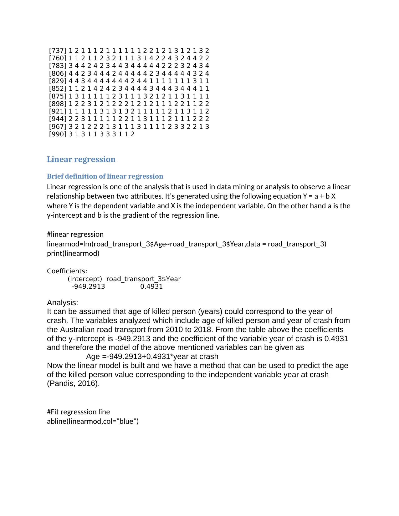
Coefficients:
(Intercept) road_transport_3$Year
-949.2913 0.4931
Analysis:
It can be assumed that age of killed person (years) could correspond to the year of
crash. The variables analyzed which include age of killed person and year of crash from
the Australian road transport from 2010 to 2018. From the table above the coefficients
of the y-intercept is -949.2913 and the coefficient of the variable year of crash is 0.4931
and therefore the model of the above mentioned variables can be given as
Age =-949.2913+0.4931*year at crash
Now the linear model is built and we have a method that can be used to predict the age
of the killed person value corresponding to the independent variable year at crash
(Pandis, 2016).
#Fit regresssion line
abline(linearmod,col="blue")
[760] 1 1 2 1 1 2 3 2 1 1 1 3 1 4 2 2 4 3 2 4 4 2 2
[783] 3 4 4 2 4 2 3 4 4 3 4 4 4 4 4 2 2 2 3 2 4 3 4
[806] 4 4 2 3 4 4 4 2 4 4 4 4 4 2 3 4 4 4 4 4 3 2 4
[829] 4 4 3 4 4 4 4 4 4 4 2 4 4 1 1 1 1 1 1 1 3 1 1
[852] 1 1 2 1 4 2 4 2 3 4 4 4 4 3 4 4 4 3 4 4 4 1 1
[875] 1 3 1 1 1 1 1 2 3 1 1 1 3 2 1 2 1 1 3 1 1 1 1
[898] 1 2 2 3 1 2 1 2 2 2 1 2 1 2 1 1 1 2 2 1 1 2 2
[921] 1 1 1 1 1 3 1 3 1 3 2 1 1 1 1 1 2 1 1 3 1 1 2
[944] 2 2 3 1 1 1 1 1 2 2 1 1 3 1 1 1 2 1 1 1 2 2 2
[967] 3 2 1 2 2 2 1 3 1 1 1 3 1 1 1 1 2 3 3 2 2 1 3
[990] 3 1 3 1 1 3 3 3 1 1 2
Linear regression
Brief definition of linear regression
Linear regression is one of the analysis that is used in data mining or analysis to observe a linear
relationship between two attributes. It’s generated using the following equation Y = a + b X
where Y is the dependent variable and X is the independent variable. On the other hand a is the
y-intercept and b is the gradient of the regression line.
#linear regression
linearmod=lm(road_transport_3$Age~road_transport_3$Year,data = road_transport_3)
print(linearmod)
Coefficients:
(Intercept) road_transport_3$Year
-949.2913 0.4931
Analysis:
It can be assumed that age of killed person (years) could correspond to the year of
crash. The variables analyzed which include age of killed person and year of crash from
the Australian road transport from 2010 to 2018. From the table above the coefficients
of the y-intercept is -949.2913 and the coefficient of the variable year of crash is 0.4931
and therefore the model of the above mentioned variables can be given as
Age =-949.2913+0.4931*year at crash
Now the linear model is built and we have a method that can be used to predict the age
of the killed person value corresponding to the independent variable year at crash
(Pandis, 2016).
#Fit regresssion line
abline(linearmod,col="blue")
#linear regression
linearmod=lm(road_transport_3$Age~road_transport_3$`Speed Limit`,data =
road_transport_3)
print(linearmod)
Coefficients:
(Intercept)
51.04627
road_transport_3$`Speed Limit`
-0.08787
Suppose we assume that the variable age of killed person (years) resulting to a higher speed limit at
location of crash. The variables analyzed are the age of killed person in years and the posted speed limit
at crash location. These variables are obtained from the Australian road death database for the years
2010 to 2018. From the data the y-intercept is 51.046 and the coefficient of the variable posted speed
limit is -0.087 (Sainami, 2013). The model is given below and it can be used to predict the age of killed
person as long as the value of the variable posted speed limit is known.
Age= 51.046-0.087*speed limit
#fit regression line
abline(linearmod,col="red")
Conclusion
In this report various patterns has been analyzed. Using the boxplot the median and the
quartile ranges has been identified for the variable age. The histogram also indicates the
frequency of the variable posted speed limit at location of crash. Using the two variable analysis
it is observed that there is no relationship between age and year of crash however the is a
relationship between age and speed limit at the location of crash.
Reflections
The linear analysis which is used for prediction will not take any input since the two variables
that are posted speed limit and age of the killed person in years are in separate subsets of data
and therefore the dataset need to be pre-processed. The best way of solving this method is to
draw a vertical line from the x value that need to be predicted. The point of interception
between the vertical line and the regression line would result to the predicted value. To avoid
future challenges or problems that may arise due to this linear analysis it is recommended to
conduct a more and thorough pre-processing of the dataset.
Secure Best Marks with AI Grader
Need help grading? Try our AI Grader for instant feedback on your assignments.
References
Aziz, M, Selim, I & Essam, A 2016, Open cluster membership probability based on K-means
clustering algorithm, Exp Astron, vol. 42, pp. 49-59 doi: 10.1007/s10686-016-9499
Sainani, K 2013, Understanding linear regression, Statistically speaking, vol. 5, pp. 10631068
doi: 10.1016/j.pmrj.2013.10.002
Pandis, N 2016, Linear regression, American Journal of Orthodontics and Dentofacial
Orthopedics, vol. 149, no. 3, pp. 431-434 doi: 10.1016/j.ajodo.2015.11.019
Lee, H, Malaspina, D, Ahn, H, Perrin, M, Opler, M, Kleinhaus, K, Harlap, S, Goetz, R & Antonius,
D 2011, Paternal age related schizophrenia (PARS): Latent subgroups detected by k-means
clustering analysis, Schizophrenia Research, vol. 128, pp. 143-149 doi:
10.1016/j.schres.2011.02.006
1 out of 11
Related Documents


Your All-in-One AI-Powered Toolkit for Academic Success.
+13062052269
info@desklib.com
Available 24*7 on WhatsApp / Email
![[object Object]](/_next/static/media/star-bottom.7253800d.svg)
Unlock your academic potential
© 2024 | Zucol Services PVT LTD | All rights reserved.