Introduction to Data Science
Added on 2022-12-29
11 Pages3150 Words22 Views
Table of Contents
Executive summary.................................................................................................... 1
Introduction................................................................................................................ 2
Data setup.................................................................................................................. 2
Exploratory data analysis........................................................................................... 2
One-variable analysis.............................................................................................. 2
Advanced analysis...................................................................................................... 6
Clustering................................................................................................................ 6
Brief explanation of k-means and clustering........................................................6
Clustering analysis.................................................................................................. 7
Linear regression..................................................................................................... 8
Brief definition of linear regression......................................................................8
Conclusion................................................................................................................ 10
Reflections................................................................................................................ 10
References............................................................................................................... 11
Introduction to data science
Executive summary
The dataset is first processed then used for analysis. The dataset from
(https://data.gov.au/data/dataset/australian-road-deaths-database ) or
blackboard will be setup and pre-processed. The following analysis will be
performed; one-variable analysis and two-variable analysis. A graph will be
provided for each analysis to enable better visualization of the mentioned
analysis. Advance analysis will also be carried out and it includes clustering
and linear regression. Clustering and k-means will be explained briefly
thereafter clustering analysis to group years will be performed. Linear
regression is explained briefly and also linear regression analysis is done and
the model plotted.
Introduction
The data analysis research report has been carried out to find out the
patterns in the study of the Australian road transport crash fatalities from
2010 to 2018. There are no specific objectives to be achieved from this
research report analysis however if anything is found to be worth studying or
significant then it will be thoroughly analyzed so as to help other
researchers, government agencies and business representatives. The given
dataset about the Australian road death fatalities will be critically analyzed.
The dataset is obtained from the blackboard or the website
(https://data.gov.au/data/dataset/australian-road-deaths-database ). The
Australian Road Death Database (ARDD) contains basic demographic and
crash details of people who died in Australia road crash. A road crash or
death means that a person dies within 30 days due to injuries obtained from
the crash. From the given dataset a value of -9 represents missing or
unknown value. The dataset consist of 20 variables or columns and some
attributes are numeric while others are string or categorical. Moreover the
Australian road transport crash fatalities from 2010 to 2018 contain 11,133
rows.
Data setup
Before the dataset is loaded into R programming, the raw
“BITREARDDFatalities.csv” file is pre-processed. Many rows are left blank or
estimated with a value of -9 to represent unrecorded or missing data. When
these values of -9 are changed using the excel replace function then cutting
these rows out will be easier in R. Now the subset of the dataset
“BITREARDDFatalities.csv” is loaded into the workspace. There is a command
getwd() in R which is used to find the location of the workspace.
> #location of workspace
> getwd()
[1] "C:/Users/JARO/Documents"
The location of the workspace is confirmed “road transport 3.xlsx” and it is
placed in the workspace location. Now that the raw data is an excel
workbook file or .xlsx which is not a text file, the built in function in R called
xlsx reader can be used to read the file information.
Exploratory data analysis
One-variable analysis
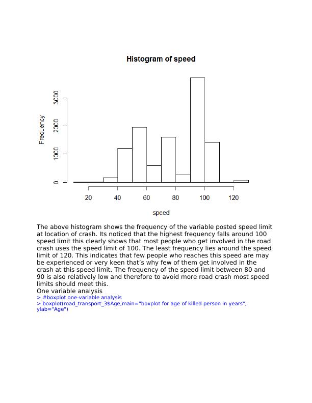
> #histogram one-variable analysis
> speed=road_transport_3$`Speed Limit`
> hist(speed)
The data analysis research report has been carried out to find out the
patterns in the study of the Australian road transport crash fatalities from
2010 to 2018. There are no specific objectives to be achieved from this
research report analysis however if anything is found to be worth studying or
significant then it will be thoroughly analyzed so as to help other
researchers, government agencies and business representatives. The given
dataset about the Australian road death fatalities will be critically analyzed.
The dataset is obtained from the blackboard or the website
(https://data.gov.au/data/dataset/australian-road-deaths-database ). The
Australian Road Death Database (ARDD) contains basic demographic and
crash details of people who died in Australia road crash. A road crash or
death means that a person dies within 30 days due to injuries obtained from
the crash. From the given dataset a value of -9 represents missing or
unknown value. The dataset consist of 20 variables or columns and some
attributes are numeric while others are string or categorical. Moreover the
Australian road transport crash fatalities from 2010 to 2018 contain 11,133
rows.
Data setup
Before the dataset is loaded into R programming, the raw
“BITREARDDFatalities.csv” file is pre-processed. Many rows are left blank or
estimated with a value of -9 to represent unrecorded or missing data. When
these values of -9 are changed using the excel replace function then cutting
these rows out will be easier in R. Now the subset of the dataset
“BITREARDDFatalities.csv” is loaded into the workspace. There is a command
getwd() in R which is used to find the location of the workspace.
> #location of workspace
> getwd()
[1] "C:/Users/JARO/Documents"
The location of the workspace is confirmed “road transport 3.xlsx” and it is
placed in the workspace location. Now that the raw data is an excel
workbook file or .xlsx which is not a text file, the built in function in R called
xlsx reader can be used to read the file information.
Exploratory data analysis
One-variable analysis
> #histogram one-variable analysis
> speed=road_transport_3$`Speed Limit`
> hist(speed)
The above histogram shows the frequency of the variable posted speed limit
at location of crash. Its noticed that the highest frequency falls around 100
speed limit this clearly shows that most people who get involved in the road
crash uses the speed limit of 100. The least frequency lies around the speed
limit of 120. This indicates that few people who reaches this speed are may
be experienced or very keen that’s why few of them get involved in the
crash at this speed limit. The frequency of the speed limit between 80 and
90 is also relatively low and therefore to avoid more road crash most speed
limits should meet this.
One variable analysis
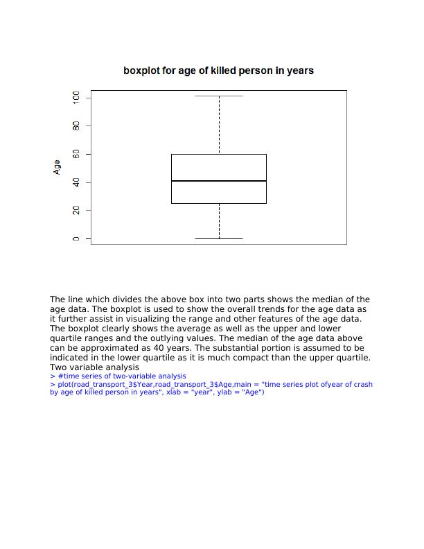
> #boxplot one-variable analysis
> boxplot(road_transport_3$Age,main="boxplot for age of killed person in years",
ylab="Age")
at location of crash. Its noticed that the highest frequency falls around 100
speed limit this clearly shows that most people who get involved in the road
crash uses the speed limit of 100. The least frequency lies around the speed
limit of 120. This indicates that few people who reaches this speed are may
be experienced or very keen that’s why few of them get involved in the
crash at this speed limit. The frequency of the speed limit between 80 and
90 is also relatively low and therefore to avoid more road crash most speed
limits should meet this.
One variable analysis
> #boxplot one-variable analysis
> boxplot(road_transport_3$Age,main="boxplot for age of killed person in years",
ylab="Age")
The line which divides the above box into two parts shows the median of the
age data. The boxplot is used to show the overall trends for the age data as
it further assist in visualizing the range and other features of the age data.
The boxplot clearly shows the average as well as the upper and lower
quartile ranges and the outlying values. The median of the age data above
can be approximated as 40 years. The substantial portion is assumed to be
indicated in the lower quartile as it is much compact than the upper quartile.
Two variable analysis
> #time series of two-variable analysis
> plot(road_transport_3$Year,road_transport_3$Age,main = "time series plot ofyear of crash
by age of killed person in years", xlab = "year", ylab = "Age")
End of preview
Want to access all the pages? Upload your documents or become a member.
Related Documents
Data Analysis Report of Australian Road Transport Crash Fatalitieslg...
|11
|3093
|79
Introduction to Data Science: Analysis of Crash Trends in Australialg...
|16
|2780
|274
Data Analysis report of Road Crasheslg...
|13
|2045
|350
Data Analysis Report of Fatalities in Australian Road Accidentslg...
|12
|2212
|59
Data Analysis Report of Fatalities in Australialg...
|16
|1986
|225
Maternal Health in Australia: Risk Factors and Analysislg...
|12
|1883
|486