Electrical Engineering Assignment Solution Analysis and Plots

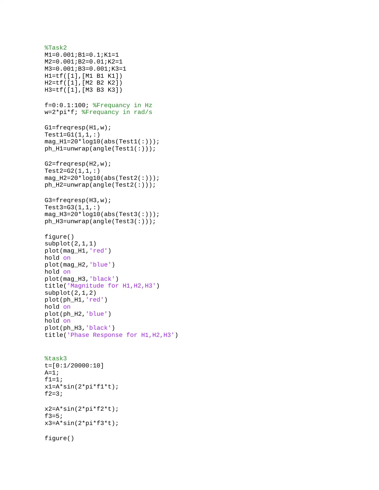
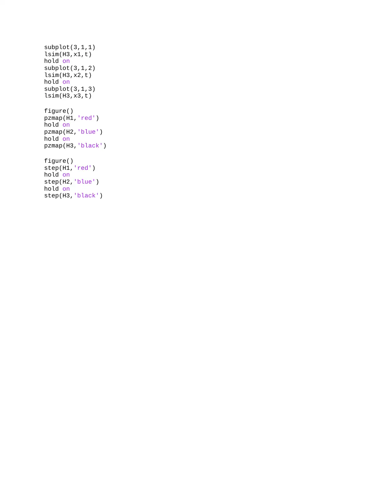
This assignment solution focuses on the analysis of different transfer functions using MATLAB. The solution includes the generation of Bode plots to visualize the frequency response of three different transfer functions (H1, H2, and H3). The magnitude and phase responses are plotted, providing insights into the system's behavior at various frequencies. Additionally, the solution involves simulating the response of H3 to sinusoidal inputs of different frequencies (1, 3, and 5 Hz) using lsim. Furthermore, the assignment includes the plotting of pole-zero maps for each transfer function and the step response analysis for the three transfer functions. The solution provides a comprehensive analysis of the systems' characteristics in both frequency and time domains, providing a complete understanding of the system's behavior.

%Task2
M1=0.001;B1=0.1;K1=1
M2=0.001;B2=0.01;K2=1
M3=0.001;B3=0.001;K3=1
H1=tf([1],[M1 B1 K1])
H2=tf([1],[M2 B2 K2])
H3=tf([1],[M3 B3 K3])
f=0:0.1:100; %Frequancy in Hz
w=2*pi*f; %Frequancy in rad/s
G1=freqresp(H1,w);
Test1=G1(1,1,:)
mag_H1=20*log10(abs(Test1(:)));
ph_H1=unwrap(angle(Test1(:)));
G2=freqresp(H2,w);
Test2=G2(1,1,:)
mag_H2=20*log10(abs(Test2(:)));
ph_H2=unwrap(angle(Test2(:)));
G3=freqresp(H3,w);
Test3=G3(1,1,:)
mag_H3=20*log10(abs(Test3(:)));
ph_H3=unwrap(angle(Test3(:)));
figure()
subplot(2,1,1)
plot(mag_H1,'red')
hold on
plot(mag_H2,'blue')
hold on
plot(mag_H3,'black')
title('Magnitude for H1,H2,H3')
subplot(2,1,2)
plot(ph_H1,'red')
hold on
plot(ph_H2,'blue')
hold on
plot(ph_H3,'black')
title('Phase Response for H1,H2,H3')
%task3
t=[0:1/20000:10]
A=1;
f1=1;
x1=A*sin(2*pi*f1*t);
f2=3;
x2=A*sin(2*pi*f2*t);
f3=5;
x3=A*sin(2*pi*f3*t);
figure()

subplot(3,1,1)
lsim(H3,x1,t)
hold on
subplot(3,1,2)
lsim(H3,x2,t)
hold on
subplot(3,1,3)
lsim(H3,x3,t)
figure()
pzmap(H1,'red')
hold on
pzmap(H2,'blue')
hold on
pzmap(H3,'black')
figure()
step(H1,'red')
hold on
step(H2,'blue')
hold on
step(H3,'black')