University Statistics Assignment: Australian Household Data Analysis
VerifiedAdded on 2020/02/24
|13
|1682
|124
Homework Assignment
AI Summary
This statistics assignment analyzes Australian household data using various statistical methods. It begins with an analysis of a sample of 200 households, employing simple random sampling to ensure unbiased data selection. The assignment presents descriptive statistics, including measures of central tendency, dispersion, and skewness, for variables such as alcohol expenditure, meals, fuel, and phone expenses. The analysis includes frequency distributions of utility expenditures, calculating percentages of households within specific spending ranges and displaying the data using histograms to illustrate skewness. Further, the assignment explores household income, calculating percentiles to identify income distributions and determining the proportion of homeowners within the sample. It also examines the relationship between total expenditure and after-tax income using correlation coefficients and scatter plots. Finally, the assignment delves into contingency tables to analyze the relationship between gender and highest degree obtained by household heads, calculating probabilities and assessing the independence of events based on the provided data.
Running head: STATISTICS
Statistics
Name of the Student
Name of the University
Author’s Note
Statistics
Name of the Student
Name of the University
Author’s Note
Paraphrase This Document
Need a fresh take? Get an instant paraphrase of this document with our AI Paraphraser
1STATISTICS
Table of Contents
Task 1...............................................................................................................................................3
Answer A.........................................................................................................................3
Answer B.........................................................................................................................3
Answer C.........................................................................................................................4
Answer D.........................................................................................................................4
Task 2...............................................................................................................................................5
Answer A.........................................................................................................................5
Answer B.........................................................................................................................5
Answer C.........................................................................................................................6
Task 3...............................................................................................................................................6
Answer A.........................................................................................................................6
Answer B.........................................................................................................................7
Answer C.........................................................................................................................7
Answer D.........................................................................................................................7
Task 4...............................................................................................................................................7
Answer A.........................................................................................................................7
Answer B.........................................................................................................................8
Answer C.........................................................................................................................8
Answer D.........................................................................................................................8
2STATISTICS
Answer E.........................................................................................................................8
References......................................................................................................................................10
Answer E.........................................................................................................................8
References......................................................................................................................................10
⊘ This is a preview!⊘
Do you want full access?
Subscribe today to unlock all pages.

Trusted by 1+ million students worldwide
3STATISTICS
Task 1
Answer A
The present assignment is an analysis of Australian Household Data. To analysis the data
a sample of 200 households were selected through the process of simple random sampling. The
process of simple random sampling was selected since the method selects the sample without any
prejudice towards the population. Moreover each and every sample in the data gets an equal
chance to get selected. The selection of the sample is based on probability method. The process
is easy to use and data from a large population can be used (Saunders, Lewis & Thornhill, 2015).
Answer B
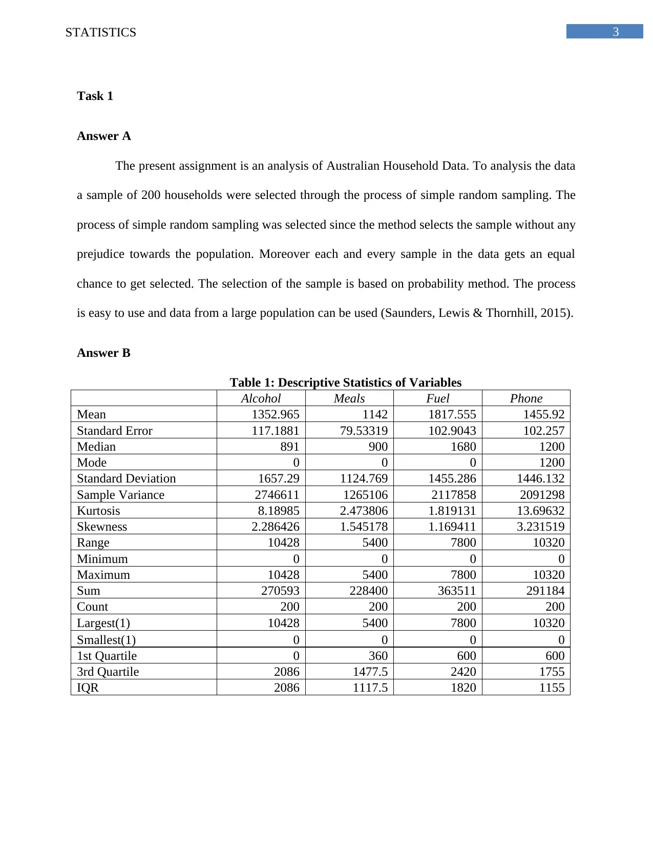
Table 1: Descriptive Statistics of Variables
Alcohol Meals Fuel Phone
Mean 1352.965 1142 1817.555 1455.92
Standard Error 117.1881 79.53319 102.9043 102.257
Median 891 900 1680 1200
Mode 0 0 0 1200
Standard Deviation 1657.29 1124.769 1455.286 1446.132
Sample Variance 2746611 1265106 2117858 2091298
Kurtosis 8.18985 2.473806 1.819131 13.69632
Skewness 2.286426 1.545178 1.169411 3.231519
Range 10428 5400 7800 10320
Minimum 0 0 0 0
Maximum 10428 5400 7800 10320
Sum 270593 228400 363511 291184
Count 200 200 200 200
Largest(1) 10428 5400 7800 10320
Smallest(1) 0 0 0 0
1st Quartile 0 360 600 600
3rd Quartile 2086 1477.5 2420 1755
IQR 2086 1117.5 1820 1155
Paraphrase This Document
Need a fresh take? Get an instant paraphrase of this document with our AI Paraphraser
4STATISTICS
Alcohol Meals Fuel Phone
-2000
-1500
-1000
-500
0
500
1000
1500
2000
2500
3000
Distribution of Expenditure
Expenditure Variables
Expenditure ($)
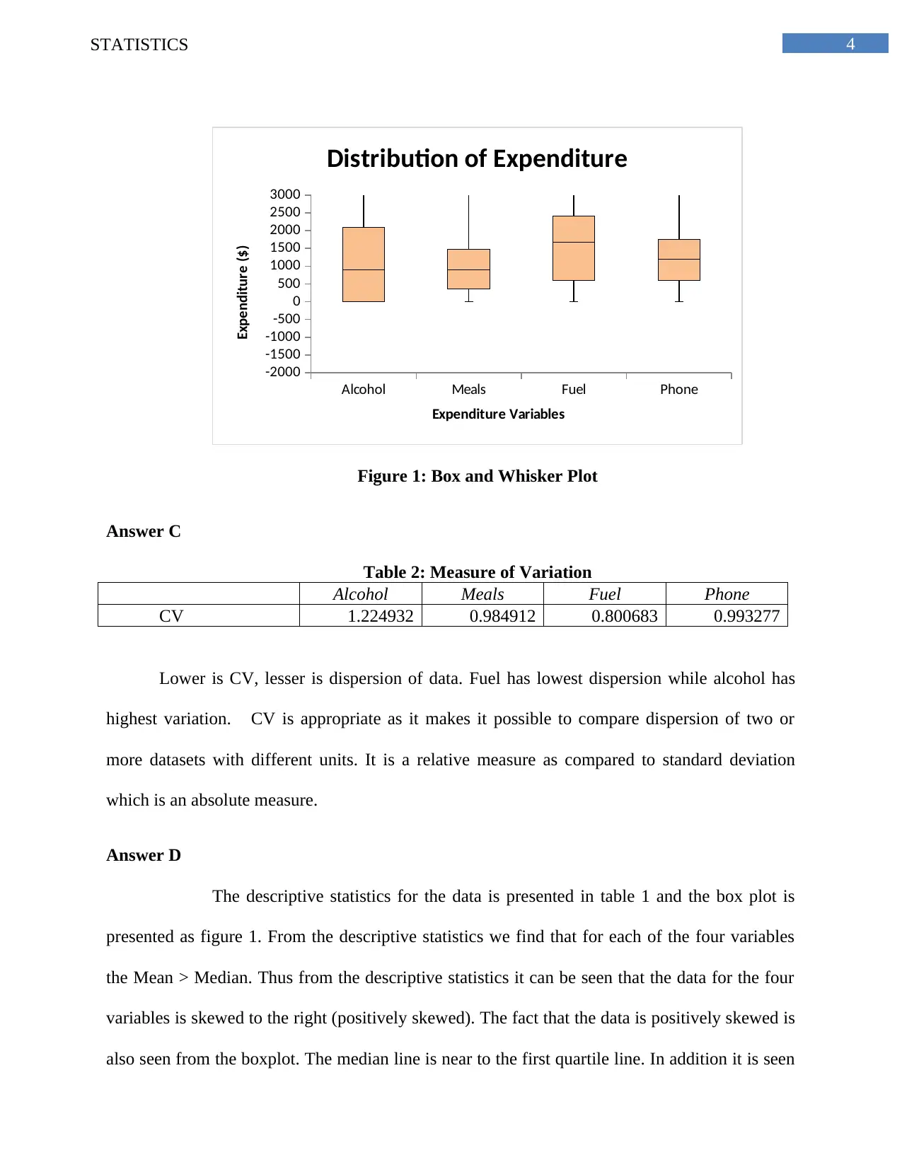
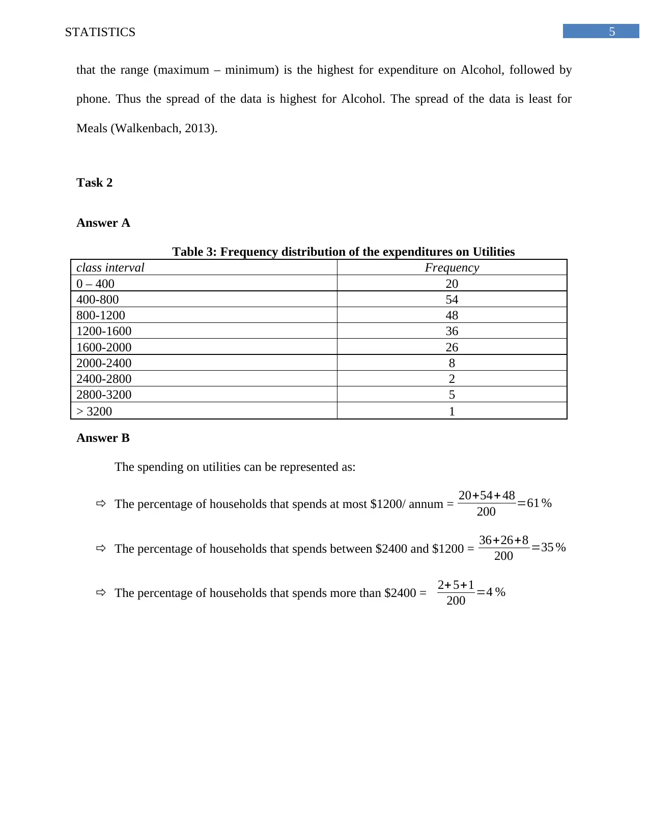
Figure 1: Box and Whisker Plot
Answer C
Table 2: Measure of Variation
Alcohol Meals Fuel Phone
CV 1.224932 0.984912 0.800683 0.993277
Lower is CV, lesser is dispersion of data. Fuel has lowest dispersion while alcohol has
highest variation. CV is appropriate as it makes it possible to compare dispersion of two or
more datasets with different units. It is a relative measure as compared to standard deviation
which is an absolute measure.
Answer D
The descriptive statistics for the data is presented in table 1 and the box plot is
presented as figure 1. From the descriptive statistics we find that for each of the four variables
the Mean > Median. Thus from the descriptive statistics it can be seen that the data for the four
variables is skewed to the right (positively skewed). The fact that the data is positively skewed is
also seen from the boxplot. The median line is near to the first quartile line. In addition it is seen
Alcohol Meals Fuel Phone
-2000
-1500
-1000
-500
0
500
1000
1500
2000
2500
3000
Distribution of Expenditure
Expenditure Variables
Expenditure ($)
Figure 1: Box and Whisker Plot
Answer C
Table 2: Measure of Variation
Alcohol Meals Fuel Phone
CV 1.224932 0.984912 0.800683 0.993277
Lower is CV, lesser is dispersion of data. Fuel has lowest dispersion while alcohol has
highest variation. CV is appropriate as it makes it possible to compare dispersion of two or
more datasets with different units. It is a relative measure as compared to standard deviation
which is an absolute measure.
Answer D
The descriptive statistics for the data is presented in table 1 and the box plot is
presented as figure 1. From the descriptive statistics we find that for each of the four variables
the Mean > Median. Thus from the descriptive statistics it can be seen that the data for the four
variables is skewed to the right (positively skewed). The fact that the data is positively skewed is
also seen from the boxplot. The median line is near to the first quartile line. In addition it is seen
5STATISTICS
that the range (maximum – minimum) is the highest for expenditure on Alcohol, followed by
phone. Thus the spread of the data is highest for Alcohol. The spread of the data is least for
Meals (Walkenbach, 2013).
Task 2
Answer A
Table 3: Frequency distribution of the expenditures on Utilities
class interval Frequency
0 – 400 20
400-800 54
800-1200 48
1200-1600 36
1600-2000 26
2000-2400 8
2400-2800 2
2800-3200 5
> 3200 1
Answer B
The spending on utilities can be represented as:
The percentage of households that spends at most $1200/ annum = 20+54+ 48
200 =61 %
The percentage of households that spends between $2400 and $1200 = 36+26+8
200 =35 %
The percentage of households that spends more than $2400 = 2+ 5+1
200 =4 %
⊘ This is a preview!⊘
Do you want full access?
Subscribe today to unlock all pages.

Trusted by 1+ million students worldwide
6STATISTICS
Answer C
0 - 400
400-800
800-1200
1200-1600
1600-2000
2000-2400
2400-2800
2800-3200
> 32000
10
20
30
40
50
60
Distribution of Expenditure on Utilities
Class Interval
Frequency
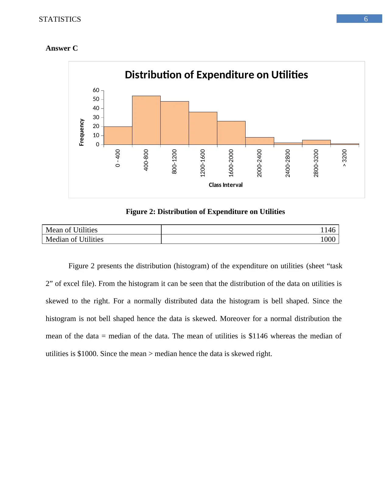
Figure 2: Distribution of Expenditure on Utilities
Mean of Utilities 1146
Median of Utilities 1000
Figure 2 presents the distribution (histogram) of the expenditure on utilities (sheet “task
2” of excel file). From the histogram it can be seen that the distribution of the data on utilities is
skewed to the right. For a normally distributed data the histogram is bell shaped. Since the
histogram is not bell shaped hence the data is skewed. Moreover for a normal distribution the
mean of the data = median of the data. The mean of utilities is $1146 whereas the median of
utilities is $1000. Since the mean > median hence the data is skewed right.
Paraphrase This Document
Need a fresh take? Get an instant paraphrase of this document with our AI Paraphraser
7STATISTICS
Task 3
Answer A
The top and bottom 10% of the household’s annual after tax income (AtaxInc) can be
represented as:
Bottom 10% = =PERCENTILE(A2:A201,0.1) = $ 18885.6
Upper 10% = =PERCENTILE(A2:A201,0.9) = $ 100401.6
The study involves a sample of 200 households. 10% means 20 households.
Thus bottom 10% signifies that 20 households have AtaxInc below $18885.6.
Similarly the Upper 10% implies that 20 households have AtaxInc above $ 100401.6.
In other words we can say that 80% of the houses have incomes that lies between
$100401.6 and $18885.6.
Answer B
There are 140 people in our sample with own house.
Thus mean of Own House = 140
200 =0.7
Based on this we can say that 70% of the people surveyed have own house.
Answer C
The number of families having size of “5” = 16.
=COUNTIF(H2:H201,5) (Triola, 2013)
Thus the probability that a randomly selected family would have a family size of 5 =
16
200 =0.08
8STATISTICS
Answer D
5 6 7 8 9 10 11 12 13 14
8
9
10
11
12
R² = 0.533174436632496
Relationship of Total expenditure
and tax income
LN(AtaxInc)
LN(Texp)
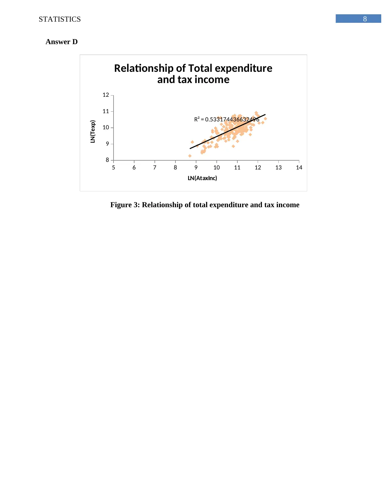
Figure 3: Relationship of total expenditure and tax income
Answer D
5 6 7 8 9 10 11 12 13 14
8
9
10
11
12
R² = 0.533174436632496
Relationship of Total expenditure
and tax income
LN(AtaxInc)
LN(Texp)
Figure 3: Relationship of total expenditure and tax income
⊘ This is a preview!⊘
Do you want full access?
Subscribe today to unlock all pages.

Trusted by 1+ million students worldwide
9STATISTICS
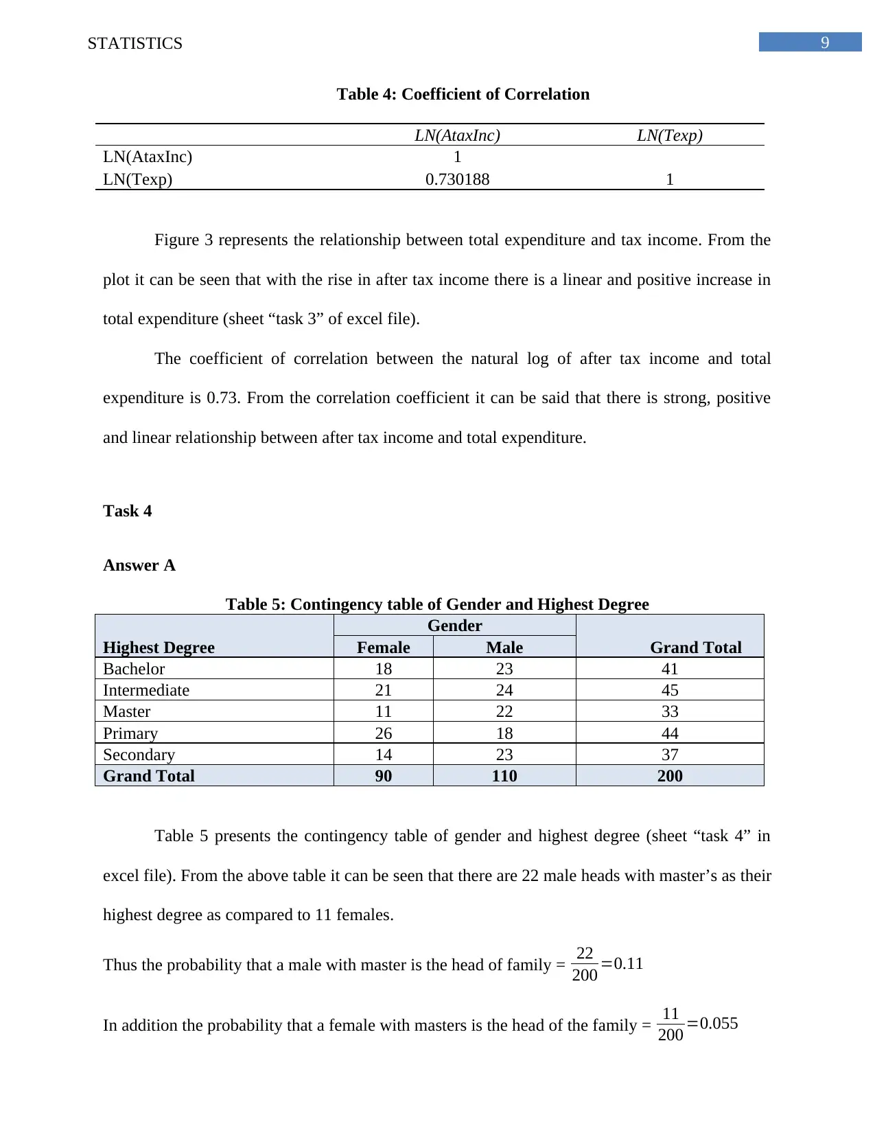
Table 4: Coefficient of Correlation
LN(AtaxInc) LN(Texp)
LN(AtaxInc) 1
LN(Texp) 0.730188 1
Figure 3 represents the relationship between total expenditure and tax income. From the
plot it can be seen that with the rise in after tax income there is a linear and positive increase in
total expenditure (sheet “task 3” of excel file).
The coefficient of correlation between the natural log of after tax income and total
expenditure is 0.73. From the correlation coefficient it can be said that there is strong, positive
and linear relationship between after tax income and total expenditure.
Task 4
Answer A
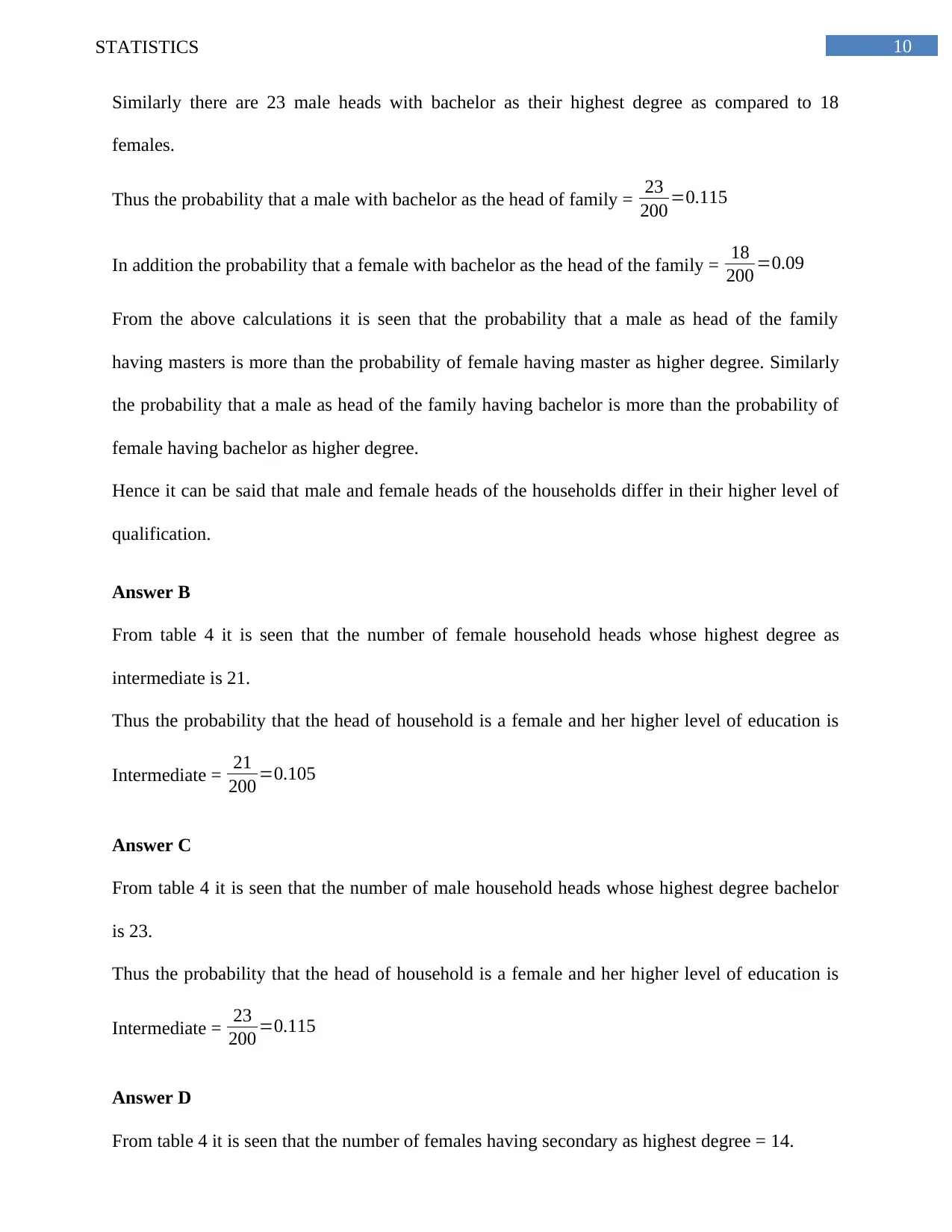
Table 5: Contingency table of Gender and Highest Degree
Highest Degree
Gender
Grand TotalFemale Male
Bachelor 18 23 41
Intermediate 21 24 45
Master 11 22 33
Primary 26 18 44
Secondary 14 23 37
Grand Total 90 110 200
Table 5 presents the contingency table of gender and highest degree (sheet “task 4” in
excel file). From the above table it can be seen that there are 22 male heads with master’s as their
highest degree as compared to 11 females.
Thus the probability that a male with master is the head of family = 22
200 =0.11
In addition the probability that a female with masters is the head of the family = 11
200 =0.055
Paraphrase This Document
Need a fresh take? Get an instant paraphrase of this document with our AI Paraphraser
10STATISTICS
Similarly there are 23 male heads with bachelor as their highest degree as compared to 18
females.
Thus the probability that a male with bachelor as the head of family = 23
200 =0.115
In addition the probability that a female with bachelor as the head of the family = 18
200 =0.09
From the above calculations it is seen that the probability that a male as head of the family
having masters is more than the probability of female having master as higher degree. Similarly
the probability that a male as head of the family having bachelor is more than the probability of
female having bachelor as higher degree.
Hence it can be said that male and female heads of the households differ in their higher level of
qualification.
Answer B
From table 4 it is seen that the number of female household heads whose highest degree as
intermediate is 21.
Thus the probability that the head of household is a female and her higher level of education is
Intermediate = 21
200 =0.105
Answer C
From table 4 it is seen that the number of male household heads whose highest degree bachelor
is 23.
Thus the probability that the head of household is a female and her higher level of education is
Intermediate = 23
200 =0.115
Answer D
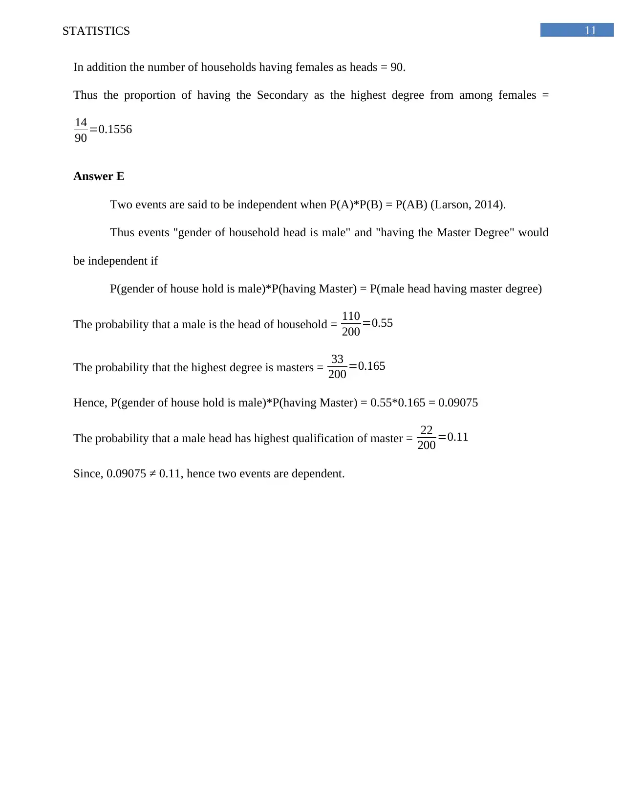
From table 4 it is seen that the number of females having secondary as highest degree = 14.
11STATISTICS
In addition the number of households having females as heads = 90.
Thus the proportion of having the Secondary as the highest degree from among females =
14
90 =0.1556
Answer E
Two events are said to be independent when P(A)*P(B) = P(AB) (Larson, 2014).
Thus events "gender of household head is male" and "having the Master Degree" would
be independent if
P(gender of house hold is male)*P(having Master) = P(male head having master degree)
The probability that a male is the head of household = 110
200 =0.55
The probability that the highest degree is masters = 33
200 =0.165
Hence, P(gender of house hold is male)*P(having Master) = 0.55*0.165 = 0.09075
The probability that a male head has highest qualification of master = 22
200 =0.11
Since, 0.09075 ≠ 0.11, hence two events are dependent.
⊘ This is a preview!⊘
Do you want full access?
Subscribe today to unlock all pages.

Trusted by 1+ million students worldwide
1 out of 13
Related Documents
Your All-in-One AI-Powered Toolkit for Academic Success.
+13062052269
info@desklib.com
Available 24*7 on WhatsApp / Email
![[object Object]](/_next/static/media/star-bottom.7253800d.svg)
Unlock your academic potential
Copyright © 2020–2026 A2Z Services. All Rights Reserved. Developed and managed by ZUCOL.


