Solved problems on thermodynamics and statistical mechanics

This article provides solutions to problems on thermodynamics and statistical mechanics, including entropy, Gibbs free energy, Carnot cycle, mixing entropy, and more. It also offers access to solved assignments, essays, and dissertations on Desklib. The solutions are presented in a step-by-step manner, making it easy for students to understand and apply the concepts.

Answer 1
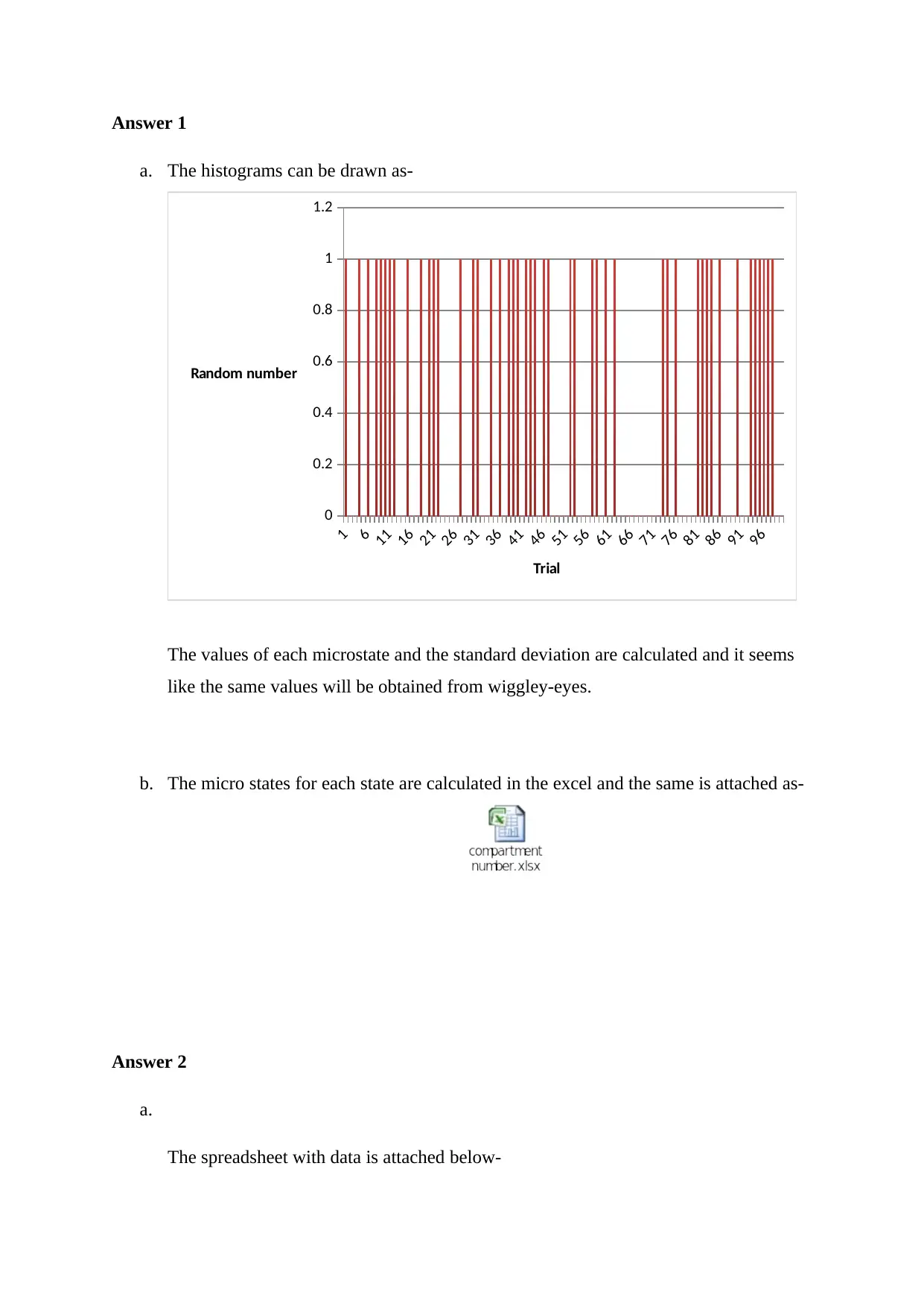
a. The histograms can be drawn as-
1
6
11
16
2126
31
36
41
46
5156
61
66
71
7681
86
91
96
0
0.2
0.4
0.6
0.8
1
1.2
Trial
Random number
The values of each microstate and the standard deviation are calculated and it seems
like the same values will be obtained from wiggley-eyes.
b. The micro states for each state are calculated in the excel and the same is attached as-
Answer 2
a.
The spreadsheet with data is attached below-

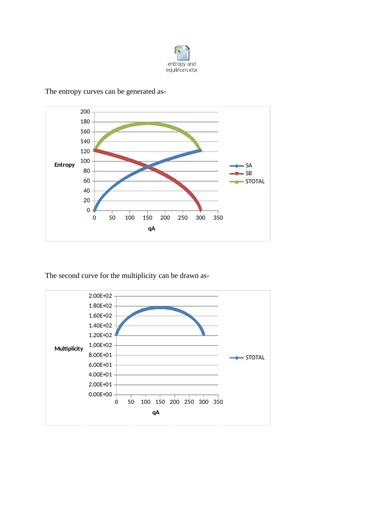
The entropy curves can be generated as-
0 50 100 150 200 250 300 350
0
20
40
60
80
100
120
140
160
180
200
SA
SB
STOTAL
qA
Entropy
The second curve for the multiplicity can be drawn as-
0 50 100 150 200 250 300 350
0.00E+00
2.00E+01
4.00E+01
6.00E+01
8.00E+01
1.00E+02
1.20E+02
1.40E+02
1.60E+02
1.80E+02
2.00E+02
STOTAL
qA
Multiplicity

b. The limitations of the spreadsheet program are as follows-
i. Calculated values may differ by standard deviation.
ii. Curve start and end point cannot be adjusted to make it more presentable.
Answer 3
Quasistatic process-
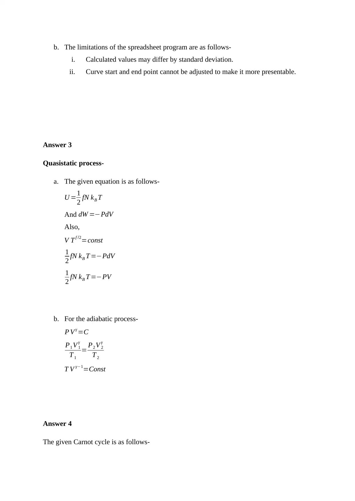
a. The given equation is as follows-
U =1
2 fN kB T
And dW =−PdV
Also,
V T f /2=const
1
2 fN kB T =−PdV
1
2 fN kB T =−PV
b. For the adiabatic process-
P V γ =C
P1 V 1
γ
T 1
= P2 V 2
γ
T 2
T V γ−1=Const
Answer 4
The given Carnot cycle is as follows-

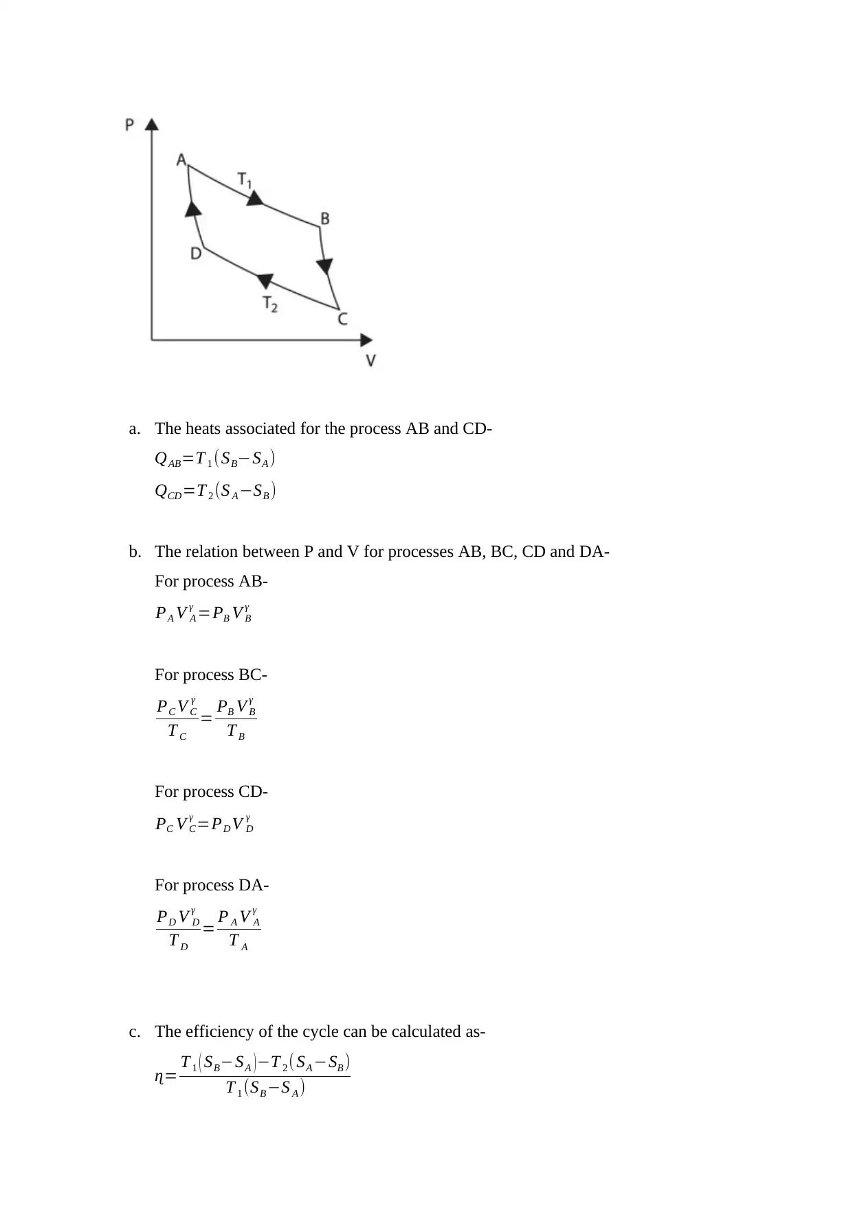
a. The heats associated for the process AB and CD-
QAB=T 1 (SB−SA )
QCD=T 2 (S A −SB )
b. The relation between P and V for processes AB, BC, CD and DA-
For process AB-
PA V A
γ =PB V B
γ
For process BC-
PC V C
γ
T C
= PB V B
γ
T B
For process CD-
PC V C
γ =PD V D
γ
For process DA-
PD V D
γ
T D
= P A V A
γ
T A
c. The efficiency of the cycle can be calculated as-
ɳ= T 1 ( SB−SA ) −T 2 ( SA −SB )
T 1 (SB −S A )

Answer 5
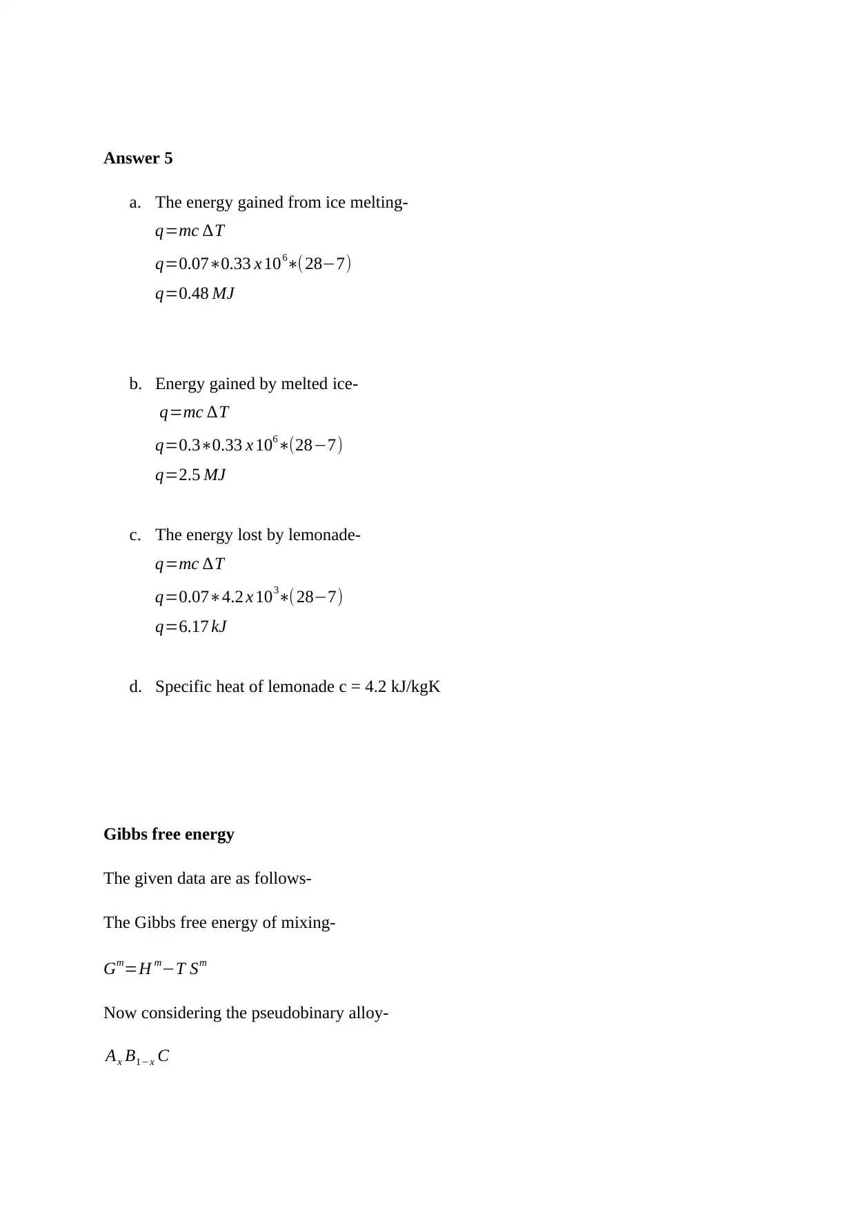
a. The energy gained from ice melting-
q=mc ∆T
q=0.07∗0.33 x 106∗(28−7)
q=0.48 MJ
b. Energy gained by melted ice-
q=mc ∆T
q=0.3∗0.33 x 106∗(28−7)
q=2.5 MJ
c. The energy lost by lemonade-
q=mc ∆T
q=0.07∗4.2 x 103∗(28−7)
q=6.17 kJ
d. Specific heat of lemonade c = 4.2 kJ/kgK
Gibbs free energy
The given data are as follows-
The Gibbs free energy of mixing-
Gm=H m−T Sm
Now considering the pseudobinary alloy-
Ax B1−x C

Part a
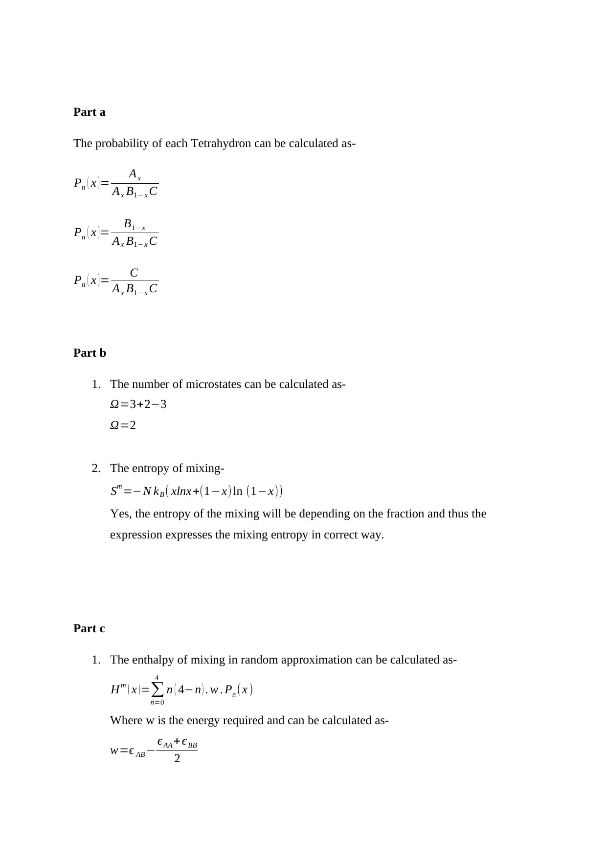
The probability of each Tetrahydron can be calculated as-
Pn ( x )= Ax
Ax B1− x C
Pn ( x ) = B1− x
Ax B1− x C
Pn ( x )= C
Ax B1− x C
Part b
1. The number of microstates can be calculated as-
Ω=3+2−3
Ω=2
2. The entropy of mixing-
Sm =−N kB ( xlnx+(1−x) ln (1−x))
Yes, the entropy of the mixing will be depending on the fraction and thus the
expression expresses the mixing entropy in correct way.
Part c
1. The enthalpy of mixing in random approximation can be calculated as-
Hm ( x )=∑
n=0
4
n ( 4−n ) . w . Pn (x )
Where w is the energy required and can be calculated as-
w=ϵ AB − ϵAA + ϵBB
2

The expression is the sum of 5 states of the random number approximation.
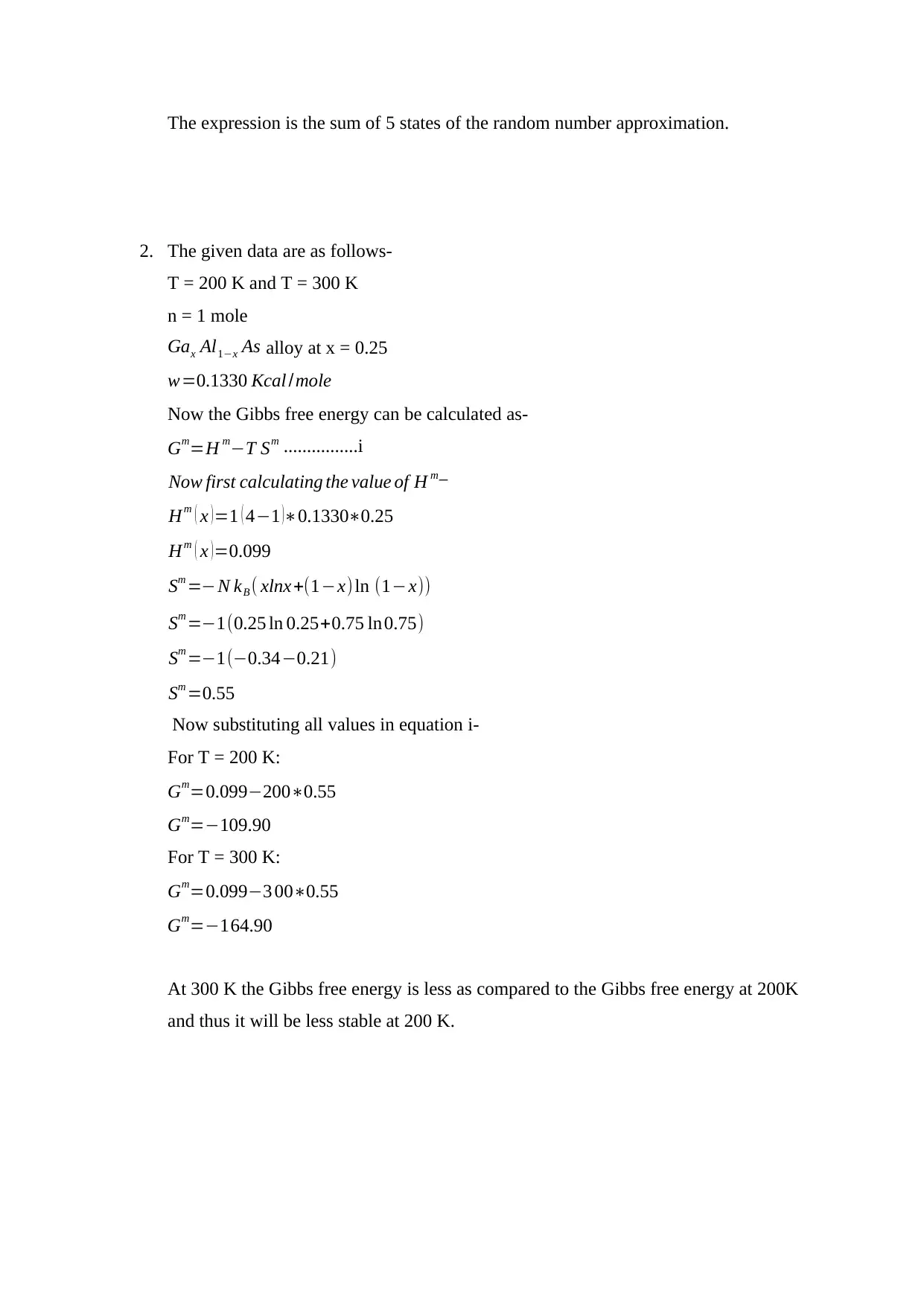
2. The given data are as follows-
T = 200 K and T = 300 K
n = 1 mole
Gax Al1−x As alloy at x = 0.25
w=0.1330 Kcal /mole
Now the Gibbs free energy can be calculated as-
Gm=H m−T Sm ................i
Now first calculating the value of H m−
Hm ( x ) =1 ( 4−1 )∗0.1330∗0.25
Hm ( x )=0.099
Sm =−N kB ( xlnx+(1−x) ln (1−x))
Sm =−1(0.25 ln 0.25+0.75 ln0.75)
Sm =−1(−0.34−0.21)
Sm =0.55
Now substituting all values in equation i-
For T = 200 K:
Gm=0.099−200∗0.55
Gm=−109.90
For T = 300 K:
Gm=0.099−3 00∗0.55
Gm=−164.90
At 300 K the Gibbs free energy is less as compared to the Gibbs free energy at 200K
and thus it will be less stable at 200 K.