HI5017 Managerial Accounting: Time-Driven vs. Driver Rate-Based ABC
VerifiedAdded on 2023/06/04
|11
|6252
|189
Report
AI Summary
This report provides an in-depth analysis of Time-Driven Activity-Based Costing (TDABC) and Driver Rate-Based Activity-Based Costing (DRBABC) methods, addressing the ongoing debate about which method is superior for assigning costs. It clarifies the differences between the 'push' and 'pull' approaches in costing, emphasizing that the choice between Time-Driven and Driver Rate-Based methods is independent of the push-pull decision. The report contrasts these methods, highlighting that both are superior to simplistic cost allocation practices. It details the mechanics of both DRBABC and TDABC, including push and pull examples, and discusses the conditions under which each method is most suitable, particularly focusing on how TDABC can provide superior information by leveraging time equations and multiple drivers to capture cost object variability. The report uses examples to illustrate the practical application of both costing methods and their impact on capacity utilization and cost recovery.
TIME-DRIVEN
OR
DRIVER
RATE-BASED
ABC:
HOW DO
YOU
CHOOSE?
OR
DRIVER
RATE-BASED
ABC:
HOW DO
YOU
CHOOSE?
Paraphrase This Document
Need a fresh take? Get an instant paraphrase of this document with our AI Paraphraser
February 2016 /STRATEGIC FINANCE/ 21
By GARY COKINS, CPIM, AND DOUGLAS D. PAUL
By GARY COKINS, CPIM, AND DOUGLAS D. PAUL
22 /STRATEGIC FINANCE/ February 2016
debate has been going on for years about
which method of activity-based costing
(ABC) is better to use for assigning costs:
Time-Driven or Driver Rate-Based. The
answer: It depends on the circum-
stances. There’s a great deal of confusion
regarding which one to use and around
terms such as “push” vs. “pull” and “top-
down” vs. “bottom-up” in which the latter perspective of
both terms is one where a product isn’t consuming all of the
supplied capacity expenses, and the former perspective is
one where the capacity expense, including unused or idle
capacity, is being fully traced into the product, thus over-
costing products. This raises several questions: How are the
approaches similar? How are they different? Is one method
superior to the other? Can a company start with the former
method and transition to the latter method as informational
needs increase? What are the conditions when one or the
other method might suffice?
To discuss the merits, we need a starting point to estab-
lish clarification. It’s an incorrect simplification to refer to
Time-Driven ABC (TDABC) as the “pull” basis and its pred-
ecessor, the conventional Driver Rate-Based ABC
(DRBABC), as the “push” approach. The decisions to use the
push vs. pull or Time-Driven vs. Driver Rate-Based method
are independent of each other, so their merits should be
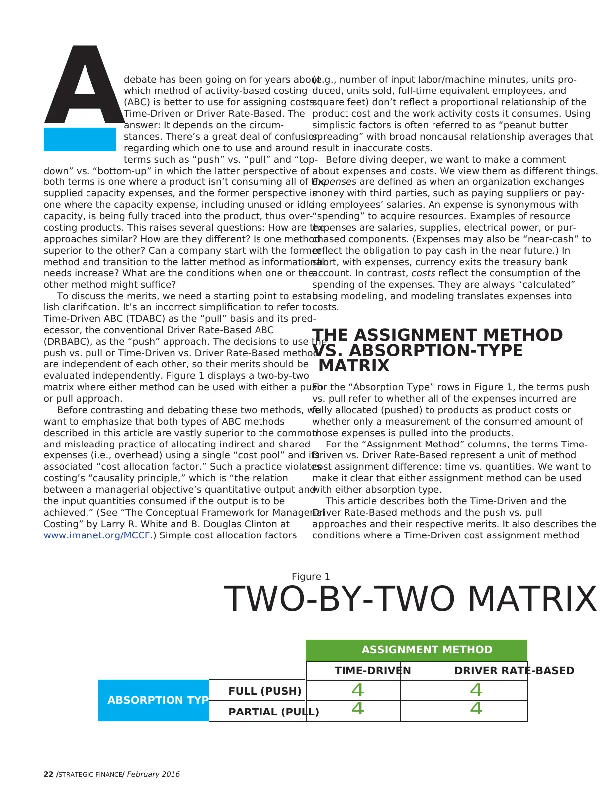
evaluated independently. Figure 1 displays a two-by-two
matrix where either method can be used with either a push
or pull approach.
Before contrasting and debating these two methods, we
want to emphasize that both types of ABC methods
described in this article are vastly superior to the common
and misleading practice of allocating indirect and shared
expenses (i.e., overhead) using a single “cost pool” and its
associated “cost allocation factor.” Such a practice violates
costing’s “causality principle,” which is “the relation
between a managerial objective’s quantitative output and
the input quantities consumed if the output is to be
achieved.” (See “The Conceptual Framework for Managerial
Costing” by Larry R. White and B. Douglas Clinton at
www.imanet.org/MCCF.) Simple cost allocation factors
(e.g., number of input labor/machine minutes, units pro-
duced, units sold, full-time equivalent employees, and
square feet) don’t reflect a proportional relationship of the
product cost and the work activity costs it consumes. Using
simplistic factors is often referred to as “peanut butter
spreading” with broad noncausal relationship averages that
result in inaccurate costs.
Before diving deeper, we want to make a comment
about expenses and costs. We view them as different things.
Expenses are defined as when an organization exchanges
money with third parties, such as paying suppliers or pay-
ing employees’ salaries. An expense is synonymous with
“spending” to acquire resources. Examples of resource
expenses are salaries, supplies, electrical power, or pur-
chased components. (Expenses may also be “near-cash” to
reflect the obligation to pay cash in the near future.) In
short, with expenses, currency exits the treasury bank
account. In contrast, costs reflect the consumption of the
spending of the expenses. They are always “calculated”
using modeling, and modeling translates expenses into
costs.
THE ASSIGNMENT METHOD
VS. ABSORPTION-TYPE
MATRIX
For the “Absorption Type” rows in Figure 1, the terms push
vs. pull refer to whether all of the expenses incurred are
fully allocated (pushed) to products as product costs or
whether only a measurement of the consumed amount of
those expenses is pulled into the products.
For the “Assignment Method” columns, the terms Time-
Driven vs. Driver Rate-Based represent a unit of method
cost assignment difference: time vs. quantities. We want to
make it clear that either assignment method can be used
with either absorption type.
This article describes both the Time-Driven and the
Driver Rate-Based methods and the push vs. pull
approaches and their respective merits. It also describes the
conditions where a Time-Driven cost assignment method
A
Figure 1
TWO-BY-TWO MATRIX
ABSORPTION TYPE
ASSIGNMENT METHOD
TIME-DRIVEN DRIVER RATE-BASED
4 4
4 4
FULL (PUSH)
PARTIAL (PULL)
ASSIGNMENT METHOD
debate has been going on for years about
which method of activity-based costing
(ABC) is better to use for assigning costs:
Time-Driven or Driver Rate-Based. The
answer: It depends on the circum-
stances. There’s a great deal of confusion
regarding which one to use and around
terms such as “push” vs. “pull” and “top-
down” vs. “bottom-up” in which the latter perspective of
both terms is one where a product isn’t consuming all of the
supplied capacity expenses, and the former perspective is
one where the capacity expense, including unused or idle
capacity, is being fully traced into the product, thus over-
costing products. This raises several questions: How are the
approaches similar? How are they different? Is one method
superior to the other? Can a company start with the former
method and transition to the latter method as informational
needs increase? What are the conditions when one or the
other method might suffice?
To discuss the merits, we need a starting point to estab-
lish clarification. It’s an incorrect simplification to refer to
Time-Driven ABC (TDABC) as the “pull” basis and its pred-
ecessor, the conventional Driver Rate-Based ABC
(DRBABC), as the “push” approach. The decisions to use the
push vs. pull or Time-Driven vs. Driver Rate-Based method
are independent of each other, so their merits should be
evaluated independently. Figure 1 displays a two-by-two
matrix where either method can be used with either a push
or pull approach.
Before contrasting and debating these two methods, we
want to emphasize that both types of ABC methods
described in this article are vastly superior to the common
and misleading practice of allocating indirect and shared
expenses (i.e., overhead) using a single “cost pool” and its
associated “cost allocation factor.” Such a practice violates
costing’s “causality principle,” which is “the relation
between a managerial objective’s quantitative output and
the input quantities consumed if the output is to be
achieved.” (See “The Conceptual Framework for Managerial
Costing” by Larry R. White and B. Douglas Clinton at
www.imanet.org/MCCF.) Simple cost allocation factors
(e.g., number of input labor/machine minutes, units pro-
duced, units sold, full-time equivalent employees, and
square feet) don’t reflect a proportional relationship of the
product cost and the work activity costs it consumes. Using
simplistic factors is often referred to as “peanut butter
spreading” with broad noncausal relationship averages that
result in inaccurate costs.
Before diving deeper, we want to make a comment
about expenses and costs. We view them as different things.
Expenses are defined as when an organization exchanges
money with third parties, such as paying suppliers or pay-
ing employees’ salaries. An expense is synonymous with
“spending” to acquire resources. Examples of resource
expenses are salaries, supplies, electrical power, or pur-
chased components. (Expenses may also be “near-cash” to
reflect the obligation to pay cash in the near future.) In
short, with expenses, currency exits the treasury bank
account. In contrast, costs reflect the consumption of the
spending of the expenses. They are always “calculated”
using modeling, and modeling translates expenses into
costs.
THE ASSIGNMENT METHOD
VS. ABSORPTION-TYPE
MATRIX
For the “Absorption Type” rows in Figure 1, the terms push
vs. pull refer to whether all of the expenses incurred are
fully allocated (pushed) to products as product costs or
whether only a measurement of the consumed amount of
those expenses is pulled into the products.
For the “Assignment Method” columns, the terms Time-
Driven vs. Driver Rate-Based represent a unit of method
cost assignment difference: time vs. quantities. We want to
make it clear that either assignment method can be used
with either absorption type.
This article describes both the Time-Driven and the
Driver Rate-Based methods and the push vs. pull
approaches and their respective merits. It also describes the
conditions where a Time-Driven cost assignment method
A
Figure 1
TWO-BY-TWO MATRIX
ABSORPTION TYPE
ASSIGNMENT METHOD
TIME-DRIVEN DRIVER RATE-BASED
4 4
4 4
FULL (PUSH)
PARTIAL (PULL)
ASSIGNMENT METHOD
⊘ This is a preview!⊘
Do you want full access?
Subscribe today to unlock all pages.
Trusted by 1+ million students worldwide
February 2016 /STRATEGIC FINANCE/ 23
provides superior information compared to
the Driver Rate-Based method.
Push vs. Pull
A push approach to costing means full
absorption in which 100% of the expenses
incurred during a time period are assigned
to the activities performed, and all of those
activity costs are in turn reassigned to the
recipients or “cost objects” that consume
them. All expenses are accounted for in
which the expenses collected in the Gen-
eral Ledger (GL) accounting system (pri-
marily from payments for purchases,
employee payroll, and accrual-type journal
entries like depreciation) equal the total
amount when adding up all of the activity
costs and the ultimate final cost object
costs. Examples of final cost objects are
products, standard service lines, types of
orders (e.g., special vs. standard or domes-
tic vs. international), channels, customers,
and business-sustaining cost objects. Other
more advanced examples of final cost
objects can include individual orders and
order lines, shipments, deliveries, medical
patient encounters (such as a visit to the
doctor), or any other type of individual
customer-related transactions. Business-
sustaining cost objects are those that aren’t
related to making products, distributing
them, or serving customers. Some people
may consider them cost assignments from
support departments (e.g., legal expenses)
and not include them with the other final
cost objects just mentioned.
The push approach proportionately
traces costs based on consumption rela-
tionships and is like a complete electrical
circuit from the provider to the receiver.
The benefit of this approach is that there’s
a 100% complete reconciliation of the
expenses to the officially reported financial
results in total. Therefore, the cost amounts
are credible overall and reasonably accu-
rate. With the push approach, estimates of
driver quantities are acceptable since each
assignment must normalize to 100%.
A downside of the push approach is
that the supplier of the resource capacity
expenses (i.e., the “sending” spender of
expenses) always recovers 100% of its
incurred expenses. Therefore, if a support
group such as information technology (IT)
or Finance spends more than its budget, it
becomes the receiving internal depart-
ment’s problem, not theirs. This doesn’t
provide an incentive to the support group
to reduce its expenses. For example, if
resources were added or paid overtime by
WHAT IS DRBABC?
Driver Rate-Based Activity-Based Costing (DRBABC) is
representative of the Activity-Based Costing (ABC) methodology that h
been formally in use to various degrees since the 1980s. It is based on
concept that assignment of costs has grown in importance because of
ever-increasing proportion of indirect and shared support expenses to
total, which, in large part, has been caused by the emergence of great
variation and complexity of product and service offerings.
DRBABC leverages operating metrics as meaningful drivers to assign
costs to “cost objects,” be they products, services, channels, or
customers. Typically, a single driver is employed in any given cost
assignment, and it’s a driver that replaces volume, revenue, or otherw
simplistic approaches.
DRBABC provides substantially higher cost accuracy compared to
traditional costing by capturing the effects of output diversity and
complexity as well as volume.
WHAT IS TDABC?Time-Driven Activity-Based Costing (TDABC) is a costing
method that reflects the supply and demand for costs and capacity th
leverages estimated unit times to calculate time as a driver in lieu of a
single driver quantity. It employs a multidriver approach to obtain an e
greater level of distinction and variability of cost between different cos
objects than DRBABC.
TDABC typically calculates costs to a more granular level, such as
transaction, invoice, order, order line, shipment, or shipment line. With
TDABC, a total time is calculated based on the rendering of an algorith
also known as a “time equation,” on every cost object record. This tim
equation allows the use of multiple drivers (as opposed to the single
DRBABC driver) with if/then logic, thus providing the flexibility to captu
more nuance and variability of a cost object’s behavior.
The TDABC methodology was presented by Steven R. Anderson and
Robert S. Kaplan in November 2004 in their article, “Time-Driven Activ
Based Costing” (Harvard Business Review, Volume 82, No. 11). The two
expanded their views in their 2007 book,Time-Driven Activity-Based
Costing, published by the Harvard Business School Press.
Paraphrase This Document
Need a fresh take? Get an instant paraphrase of this document with our AI Paraphraser
24 /STRATEGIC FINANCE/ February 2016
$ # Invoices Rate $ # Invoices Rate
Salaries $100,000 $98,000
Benefits $30,000 $28,900
Training $7,000 $4,200
Travel $8,000 $3,000
Allocations In $20,000 $19,800
Subtotal - All Costs In $$1$16$165$165,$165,0$165,00$165,000$165,000 $153,900
Customer 1 $41,420 33,136 $1.25 $41,820 33,456 $1.25
Customer 2 $39,420 31,536 $1.25 $61,155 48,924 $1.25
Customer 3 $36,545 29,236 $1.25 $34,016 27,213 $1.25
Customer 4 $34,920 27,936 $1.25 $20,918 16,734 $1.25
Subtotal - Recovery to Customers $
$165,000
$1
$165,000
$15
$165,000
$152
$165,000
$152,
$165,000
$152,3
$165,000
$152,30
$165,000
$152,305
$165,000
$152,305 121,844 $1.25 $157,909 126,327 $1.25
Net Over/(Under) Recovery (
$165,000
$152,305
($
$165,000
$152,305
($1
$165,000
$152,305
($12
$165,000
$152,305
($12,
$165,000
$152,305
($12,6
$165,000
$152,305
($12,69
$165,000
$152,305
($12,695
$165,000
$152,305
($12,695)
$165,000
$152,305
($12,695) $4,009
Capacity Utilization (Recovery/Total Spent) 9
$165,000
$152,305
($12,695)
92
$165,000
$152,305
($12,695)
92.
$165,000
$152,305
($12,695)
92.3
$165,000
$152,305
($12,695)
92.3%
$165,000
$152,305
($12,695)
92.3% 102.6%
January February
Accounts Receivable Department
Activity - Manage Invoices
$ # Invoices Driver % Net Rate $ # Invoices Driver % Net Rate
Salaries $100,000 $98,000
Benefits $30,000 $28,900
Training $7,000 $4,200
Travel $8,000 $3,000
Allocations In $20,000 $19,800
Subtotal - All Costs In $$1$16$165$165,$165,0$165,00$165,000$165,000 $153,900
Customer 1 $44,872 33,136 27.2% $1.35 $40,758 33,456 26.5% $1.22
Customer 2 $42,706 31,536 25.9% $1.35 $59,602 48,924 38.7% $1.22
Customer 3 $39,591 29,236 24.0% $1.35 $33,153 27,213 21.5% $1.22
Customer 4 $37,831 27,936 22.9% $1.35 $20,386 16,734 13.2% $1.22
Subtotal - Recovery to Customers $
$165,000
$1
$165,000
$16
$165,000
$165
$165,000
$165,
$165,000
$165,0
$165,000
$165,00
$165,000
$165,000
$165,000
$165,000 121,844 100% $1.35 $153,900 126,327 $1.22
Net Over/(Under) Recovery $
$165,000
$165,000
$0
$165,000
$165,000
$0 $0
Capacity Utilization (Recovery/Total Spent) 1
$165,000
$165,000
$0
10
$165,000
$165,000
$0
100
$165,000
$165,000
$0
100.
$165,000
$165,000
$0
100.0
$165,000
$165,000
$0
100.0%
$165,000
$165,000
$0
100.0% 100.0%
Accounts Receivable Department
Activity - Manage Invoices
January February
Department Activity Period Amount Time Equation
Accounts Receivable Manage Invoices January $$1$16$165$165,$165,0$165,00$165,000$165,000 If [Invoice].[Order Type]="Web", Then 1 Else if [Invoice].[Order Type]="Fax" Then 5 Else 8
Headcount Hours Per Head Available Hours Available Minutes
65 8 10,400 624,000 Invoice ID Business Group ID Order Type Count Time Cost
2016-01-000001 Customer 1 Web 1 1 $0.30
2016-01-000002 Customer 2 Web 1 1 $0.30
2016-01-000003 Customer 3 Fax 1 5 $1.49
2016-01-000004 Customer 1 Phone 1 8 $2.39
2016-01-000005 Customer 4 Web 1 1 $0.30
2016-01-000006 Customer 2 Phone 1 8 $2.39
2016-01-000007 Customer 4 Web 1 1 $0.30
……. Customer 1 Web 15,078 15,078 $4,506.19
……. Customer 2 Web 13,078 13,078 $3,908.47
$165,000$165,000$165,000$165,000$165,000$165,000$165,000$165,000$165,000$165,000$165,000$165,000$165,000$165,000
……. Customer 3 Web 8,578 8,578 $2,563.61
……. Customer 4 Web 11,078 11,078 $3,310.75
……. Customer 1 Fax 8,078 40,390 $12,070.89
……. Customer 2 Fax 7,078 35,390 $10,576.60
……. Customer 3 Fax 7,578 37,890 $11,323.74
……. Customer 4 Fax 6,578 32,890 $9,829.45
……. Customer 1 Phone 9,978 79,824 $23,856.07
……. Customer 2 Phone 11,378 91,024 $27,203.28
……. Customer 3 Phone 13,078 104,624 $31,267.76
……. Customer 4 Phone 10,278 82,224 $24,573.33
2016-01-121843 Customer 3 Phone 1 8 $2.39
Total 121,844 552,101 $
$165,000
$1
$165,000
$16
$165,000
$165
$165,000
$165,
$165,000
$165,0
$165,000
$165,00
$165,000
$165,000
$165,000
$165,000
Capacity Utilization (Total Time/Available Minutes) 8
$165,000
$165,000
88
$165,000
$165,000
88.
$165,000
$165,000
88.5
$165,000
$165,000
88.5%
$165,000
$165,000
88.5%
Table 1
DRBABC PULL EXAMPLE
Table 2
DRBABC PUSH EXAMPL
Table 3
TDABC EXAMPLE
($12,695)
February 2016 /STRATEGIC FINANCE/ 25
IT or Finance to meet deadlines or performance measures,
those receiving the allocation would bear the cost impact,
no matter whose behavior caused the variance. Another
negative aspect of the push approach is that it is frequently
capacity insensitive. That is, there’s no obvious way to dif-
ferentiate and classify individual resource capacities as used
or unused (e.g., idle or excess). Hence, the final cost objects
will be modestly overcosted for expenses that they didn’t
cause or require.
As a result of the shortcomings of the push approach, the
pull approach was born. Think of it as a partial absorption
of the resources’ expenses. With the pull approach, senders
of expenses can be viewed as mini profit centers in which
agreed-upon rates for their services are established, typi-
cally based on a budget of planned expenses and expected
volumes. Consumers of these services pay a fixed rate (i.e.,
price) for the actual volume that they consume—no more,
no less. The pull approach opens a new world of arm’s-
length relationships between supporting centers and
customer-facing departments. Customers, whether they are
internal or external, often prefer this arrangement because
it allows them to have some control over how much
expense from their organization is planned for them as
costs.
Additionally, internal service providers may favor this
method because it can show the value of their services or the
need for additional resources based on the overrecovery or
underrecovery of their costs charged to their customers. For
example, if an IT group were shown to be overrecovering its
costs via these chargeouts by a large margin, this information
could be used as justification for increased headcount or at
least demonstrate that they are performing highly. The pull
approach also introduces a rudimentary measure of capacity
utilization: the percent over/under cost recovery. But a prob-
lem with the pull approach is that the correctness of the cost
assignment is highly contingent on setting accurate rates.
Imagine a cost assignment network that includes cross-
charging in which estimated rates are applied. There would
be multiple overrecoveries and underrecoveries of expenses,
potentially large ones, because of faulty rates. The result
would be a difference from the actual GL expense totals in
aggregate, thereby questioning the overall credibility and
understanding of the costs.
Time-Driven vs. Driver Rate-Based
Regardless of the previously referenced advantages and dis-
advantages of the push- vs. pull-based costing approaches,
there lies a separate decision as to whether to use TDABC or
use the conventional DRBABC assignments. Both methods
can be used with either a push or pull approach. To see
how, consider the following examples.
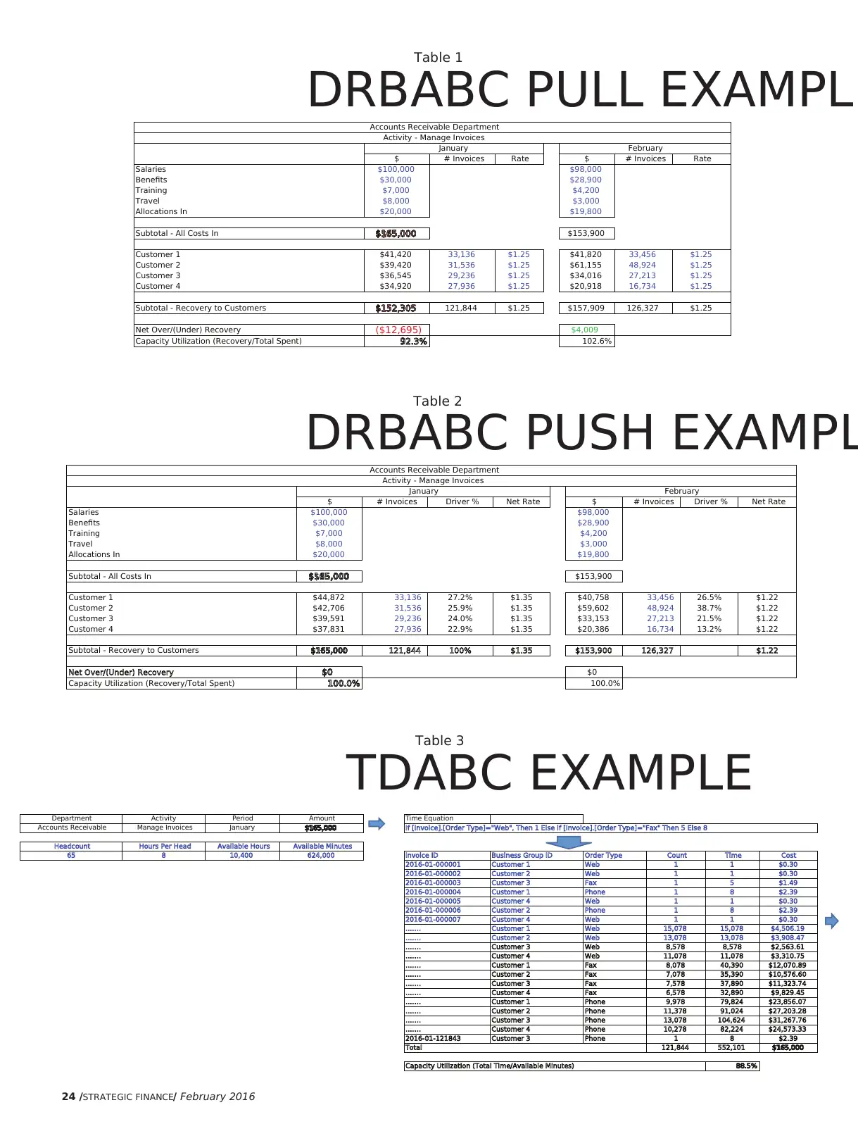
DRIVER RATE-BASED ABC
Pull Approach. An Accounts Receivable (A/R) department
could establish an activity cost driver that is a predefined
rate, such as $1.25 per invoice, based on its budget and vol-
ume projections, and charge for its services on that basis.
At the end of the year, the A/R department will be over-
recovered or underrecovered because their actual incurred
expenses and the volume consumed will never match the
projection exactly, no matter how skilled an organization is
at budgeting. In this example, the pull approach’s driver is
the quantity-based number of invoices rather than a stan-
dard time to process each invoice.
You can see a shortcoming of the pull approach in
Table 1. While a form of capacity utilization value is an out-
put from this approach, there’s a financial underrecovery in
January and an overrecovery in February. The total amount
spent in January was $165,000, but only $152,305 was
charged to customers. In February, $157,909 was charged,
but only $153,900 was spent.
These differences would eventually need to be recon-
ciled somehow at some point.
Push Approach. Alternatively, the DRBABC method could
be used with a push approach in which all of the A/R
department expenses are charged to customers. No over-
recovery or underrecovery reconciliation would be
required. See Table 2 in which all of the expenses are
charged as costs based on number of invoices, resulting in a
net calculated rate each month.
In this case, all of the $165,000 January expenses and all
of the $153,900 February expenses are charged to cus-
tomers, thereby resolving the financial variance problem.
Yet note that the capacity utilization is always 100%. The
cost rate was different in each month, and there’s no meas-
ure of the efficiency of the department.
TIME-DRIVEN ABC
TDABC is a model of supply and demand for cost and
capacity that leverages estimated unit times, not unit quan-
tities. It solves some of the challenges in DRBABC because it
can provide both a full assignment of the expenses as costs
and a meaningful capacity utilization measure. Consider
that the same A/R department could utilize a time-driven
assignment method that’s dependent on the unit times to
process the various types of invoices, which means the
time will differ whether the invoices were received via
Web, fax, or phone. These time-based variables are cap-
tured in a formula that calculates the amount of time taken
to process each invoice. With TDABC, the total time is cal-
culated based on rendering the time equation on every
invoice. The actual A/R department dollars then get
charged to each invoice based on an individual invoice’s
$ % Invoices Net Rate
Customer 1 $40,436 24.5% 33,136 $1.22
Customer 2 $41,691 25.3% 31,536 $1.32
Customer 3 $45,159 27.4% 29,236 $1.54
Customer 4 $37,714 22.9% 27,936 $1.35
Total $$1$16$165$165,$165,0$165,00$165,000$165,000 1$165,000 10$165,000 100$165,000 100.$165,000 100.0$165,000 100.0%$165,000 100.0% 121,844 $1.35$165,000 100.0%$165,000 100.0%$165,000 100.0%$165,000 100.0%$165,000 100.0%$165,000 100.0%$165,000 100.0%$165,000 100.0%$165,000 100.0%$165,000 100.0%$165,000 100.0%$165,000 100.0%$165,000 100.0%
IT or Finance to meet deadlines or performance measures,
those receiving the allocation would bear the cost impact,
no matter whose behavior caused the variance. Another
negative aspect of the push approach is that it is frequently
capacity insensitive. That is, there’s no obvious way to dif-
ferentiate and classify individual resource capacities as used
or unused (e.g., idle or excess). Hence, the final cost objects
will be modestly overcosted for expenses that they didn’t
cause or require.
As a result of the shortcomings of the push approach, the
pull approach was born. Think of it as a partial absorption
of the resources’ expenses. With the pull approach, senders
of expenses can be viewed as mini profit centers in which
agreed-upon rates for their services are established, typi-
cally based on a budget of planned expenses and expected
volumes. Consumers of these services pay a fixed rate (i.e.,
price) for the actual volume that they consume—no more,
no less. The pull approach opens a new world of arm’s-
length relationships between supporting centers and
customer-facing departments. Customers, whether they are
internal or external, often prefer this arrangement because
it allows them to have some control over how much
expense from their organization is planned for them as
costs.
Additionally, internal service providers may favor this
method because it can show the value of their services or the
need for additional resources based on the overrecovery or
underrecovery of their costs charged to their customers. For
example, if an IT group were shown to be overrecovering its
costs via these chargeouts by a large margin, this information
could be used as justification for increased headcount or at
least demonstrate that they are performing highly. The pull
approach also introduces a rudimentary measure of capacity
utilization: the percent over/under cost recovery. But a prob-
lem with the pull approach is that the correctness of the cost
assignment is highly contingent on setting accurate rates.
Imagine a cost assignment network that includes cross-
charging in which estimated rates are applied. There would
be multiple overrecoveries and underrecoveries of expenses,
potentially large ones, because of faulty rates. The result
would be a difference from the actual GL expense totals in
aggregate, thereby questioning the overall credibility and
understanding of the costs.
Time-Driven vs. Driver Rate-Based
Regardless of the previously referenced advantages and dis-
advantages of the push- vs. pull-based costing approaches,
there lies a separate decision as to whether to use TDABC or
use the conventional DRBABC assignments. Both methods
can be used with either a push or pull approach. To see
how, consider the following examples.
DRIVER RATE-BASED ABC
Pull Approach. An Accounts Receivable (A/R) department
could establish an activity cost driver that is a predefined
rate, such as $1.25 per invoice, based on its budget and vol-
ume projections, and charge for its services on that basis.
At the end of the year, the A/R department will be over-
recovered or underrecovered because their actual incurred
expenses and the volume consumed will never match the
projection exactly, no matter how skilled an organization is
at budgeting. In this example, the pull approach’s driver is
the quantity-based number of invoices rather than a stan-
dard time to process each invoice.
You can see a shortcoming of the pull approach in
Table 1. While a form of capacity utilization value is an out-
put from this approach, there’s a financial underrecovery in
January and an overrecovery in February. The total amount
spent in January was $165,000, but only $152,305 was
charged to customers. In February, $157,909 was charged,
but only $153,900 was spent.
These differences would eventually need to be recon-
ciled somehow at some point.
Push Approach. Alternatively, the DRBABC method could
be used with a push approach in which all of the A/R
department expenses are charged to customers. No over-
recovery or underrecovery reconciliation would be
required. See Table 2 in which all of the expenses are
charged as costs based on number of invoices, resulting in a
net calculated rate each month.
In this case, all of the $165,000 January expenses and all
of the $153,900 February expenses are charged to cus-
tomers, thereby resolving the financial variance problem.
Yet note that the capacity utilization is always 100%. The
cost rate was different in each month, and there’s no meas-
ure of the efficiency of the department.
TIME-DRIVEN ABC
TDABC is a model of supply and demand for cost and
capacity that leverages estimated unit times, not unit quan-
tities. It solves some of the challenges in DRBABC because it
can provide both a full assignment of the expenses as costs
and a meaningful capacity utilization measure. Consider
that the same A/R department could utilize a time-driven
assignment method that’s dependent on the unit times to
process the various types of invoices, which means the
time will differ whether the invoices were received via
Web, fax, or phone. These time-based variables are cap-
tured in a formula that calculates the amount of time taken
to process each invoice. With TDABC, the total time is cal-
culated based on rendering the time equation on every
invoice. The actual A/R department dollars then get
charged to each invoice based on an individual invoice’s
$ % Invoices Net Rate
Customer 1 $40,436 24.5% 33,136 $1.22
Customer 2 $41,691 25.3% 31,536 $1.32
Customer 3 $45,159 27.4% 29,236 $1.54
Customer 4 $37,714 22.9% 27,936 $1.35
Total $$1$16$165$165,$165,0$165,00$165,000$165,000 1$165,000 10$165,000 100$165,000 100.$165,000 100.0$165,000 100.0%$165,000 100.0% 121,844 $1.35$165,000 100.0%$165,000 100.0%$165,000 100.0%$165,000 100.0%$165,000 100.0%$165,000 100.0%$165,000 100.0%$165,000 100.0%$165,000 100.0%$165,000 100.0%$165,000 100.0%$165,000 100.0%$165,000 100.0%
⊘ This is a preview!⊘
Do you want full access?
Subscribe today to unlock all pages.
Trusted by 1+ million students worldwide
26 /STRATEGIC FINANCE/ February 2016
processing time relative to the total processing time of all
invoices. (See Time-Driven Activity-Based Costing by Robert S.
Kaplan and Steven R. Anderson, p. 36, for more details on
this technique for the cost calculations.) This is time-driven
because it uses a time algorithm applied to each transaction
and push because all the expenses are accounted for.
TDABC’s time algorithms are also referred to as time
equations.
With TDABC, the costs are calculated at the invoice level
of detail, not at the aggregated customer level (see Table 3).
The time equation is applied at that more granular level,
and the total amount allocated matches the incurred
expenses, i.e., the same $165,000 in January as seen previ-
ously. The total invoice count matches the total in the con-
ventional DRBABC example, but in this case all of the
dollars were pushed and a calculated time was the basis for
the assignment.
It’s important to realize that the time calculation was
based on the input of standard unit times for the different
order types, not actual times clocked or estimated times
surveyed.
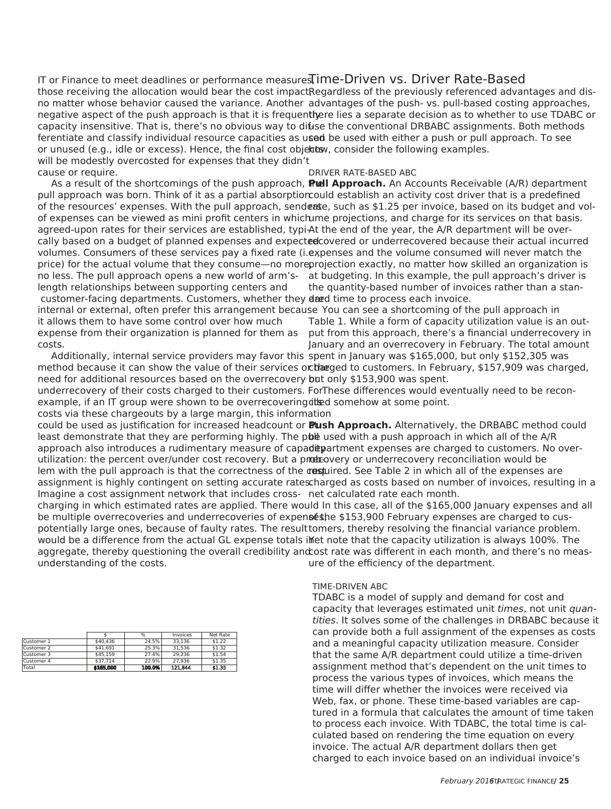
When the values for January are aggregated by cus-
tomer, the summed amounts for each customer are differ-
ent than they were for the DRBABC approach because the
time-driven approach captures more variation and diversity
of cost objects. Customer 3’s low use of Web and high use of
phone increased its cost and provided insight that wouldn’t
be found using the single-driver case. The DRBABC method
can address this by further disaggregating the activity into
more granular ones. But this introduces the issue of how
granular and detailed the DRBABC model and its associated
data collection of activity driver quantities should be
designed. We discuss this issue later in the article.
Additionally, note that there’s a capacity utilization meas-
ure in this full absorption push approach. The DRBABC full
absorption case was capacity insensitive (i.e., 100% of capac-
ity is utilized). The pull single-rate DRBABC approach
showed 92% capacity utilization based on the somewhat
arbitrary standard rate vs. the more informed fact-based
89% utilization using the time-driven method. The
consumed-capacity value from the TDABC approach is based
on the grand total time that was calculated and used to allo-
cate the cost. The available capacity is calculated based on
the number of full-time equivalents (FTEs) multiplied by the
available hours per FTE, two frequently known or estimable
values. This ratio of these two amounts is the capacity uti-
lization, which can be greater or less than 100%. (See Kaplan
and Anderson, p. 77, for an implementation example using
this technique for calculating capacity utilization.)
ABC MODEL STRUCTURE
IMPLICATIONS:
THE CROSSOVER POINT
In defense of the DRBABC approach, the “variation and
diversity” captured by the TDABC approach in the previous
A/R department example could also have been detected
and captured with DRBABC’s push approach through some
additional work. As described earlier, this would have
required “disaggregating” (i.e., decomposing the A/R
department’s activity dictionary into more granular activi-
ties). It will also require estimates from one or more
employees in the A/R department for the increased number
of resource assignments to calculate the activity costs. (An
activity dictionary is a list of activities by function, depart-
ment, and business process that managers can use to help
determine key metrics and find ways to improve opera-
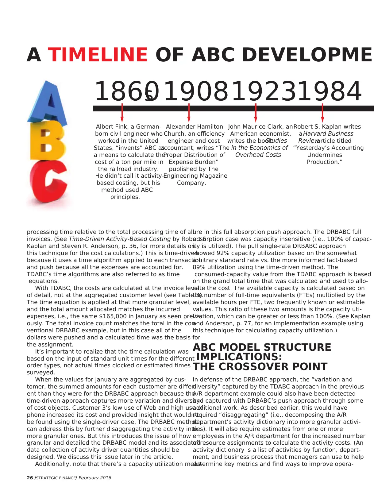
1860s
Albert Fink, a German-
born civil engineer who
worked in the United
States, “invents” ABC as
a means to calculate the
cost of a ton per mile in
the railroad industry.
He didn’t call it activity-
based costing, but his
method used ABC
principles.
1908
Alexander Hamilton
Church, an efficiency
engineer and cost
accountant, writes “The
Proper Distribution of
Expense Burden”
published by The
Engineering Magazine
Company.
1923
John Maurice Clark, an
American economist,
writes the bookStudies
in the Economics of
Overhead Costs.
1984
Robert S. Kaplan writes
a Harvard Business
Reviewarticle titled
“Yesterday’s Accounting
Undermines
Production.”
A TIMELINE OF ABC DEVELOPMEN
processing time relative to the total processing time of all
invoices. (See Time-Driven Activity-Based Costing by Robert S.
Kaplan and Steven R. Anderson, p. 36, for more details on
this technique for the cost calculations.) This is time-driven
because it uses a time algorithm applied to each transaction
and push because all the expenses are accounted for.
TDABC’s time algorithms are also referred to as time
equations.
With TDABC, the costs are calculated at the invoice level
of detail, not at the aggregated customer level (see Table 3).
The time equation is applied at that more granular level,
and the total amount allocated matches the incurred
expenses, i.e., the same $165,000 in January as seen previ-
ously. The total invoice count matches the total in the con-
ventional DRBABC example, but in this case all of the
dollars were pushed and a calculated time was the basis for
the assignment.
It’s important to realize that the time calculation was
based on the input of standard unit times for the different
order types, not actual times clocked or estimated times
surveyed.
When the values for January are aggregated by cus-
tomer, the summed amounts for each customer are differ-
ent than they were for the DRBABC approach because the
time-driven approach captures more variation and diversity
of cost objects. Customer 3’s low use of Web and high use of
phone increased its cost and provided insight that wouldn’t
be found using the single-driver case. The DRBABC method
can address this by further disaggregating the activity into
more granular ones. But this introduces the issue of how
granular and detailed the DRBABC model and its associated
data collection of activity driver quantities should be
designed. We discuss this issue later in the article.
Additionally, note that there’s a capacity utilization meas-
ure in this full absorption push approach. The DRBABC full
absorption case was capacity insensitive (i.e., 100% of capac-
ity is utilized). The pull single-rate DRBABC approach
showed 92% capacity utilization based on the somewhat
arbitrary standard rate vs. the more informed fact-based
89% utilization using the time-driven method. The
consumed-capacity value from the TDABC approach is based
on the grand total time that was calculated and used to allo-
cate the cost. The available capacity is calculated based on
the number of full-time equivalents (FTEs) multiplied by the
available hours per FTE, two frequently known or estimable
values. This ratio of these two amounts is the capacity uti-
lization, which can be greater or less than 100%. (See Kaplan
and Anderson, p. 77, for an implementation example using
this technique for calculating capacity utilization.)
ABC MODEL STRUCTURE
IMPLICATIONS:
THE CROSSOVER POINT
In defense of the DRBABC approach, the “variation and
diversity” captured by the TDABC approach in the previous
A/R department example could also have been detected
and captured with DRBABC’s push approach through some
additional work. As described earlier, this would have
required “disaggregating” (i.e., decomposing the A/R
department’s activity dictionary into more granular activi-
ties). It will also require estimates from one or more
employees in the A/R department for the increased number
of resource assignments to calculate the activity costs. (An
activity dictionary is a list of activities by function, depart-
ment, and business process that managers can use to help
determine key metrics and find ways to improve opera-
1860s
Albert Fink, a German-
born civil engineer who
worked in the United
States, “invents” ABC as
a means to calculate the
cost of a ton per mile in
the railroad industry.
He didn’t call it activity-
based costing, but his
method used ABC
principles.
1908
Alexander Hamilton
Church, an efficiency
engineer and cost
accountant, writes “The
Proper Distribution of
Expense Burden”
published by The
Engineering Magazine
Company.
1923
John Maurice Clark, an
American economist,
writes the bookStudies
in the Economics of
Overhead Costs.
1984
Robert S. Kaplan writes
a Harvard Business
Reviewarticle titled
“Yesterday’s Accounting
Undermines
Production.”
A TIMELINE OF ABC DEVELOPMEN
Paraphrase This Document
Need a fresh take? Get an instant paraphrase of this document with our AI Paraphraser
February 2016 /STRATEGIC FINANCE/ 27
tions.) For example, the original activity “process invoices”
would be subdivided into “process invoices by the Web”
and “process invoices by phone.” Each customer A to D
would then be charged based on the number of types of
processed invoices (i.e., the activity cost driver).
The level of disaggregation of activities defined with a
DRBABC model to match desired cost accuracy require-
ments begins to provide some insights as to how and why
TDABC is different from DRBABC. Increasing disaggregation
requires both an increased number of resource expense
assignments to the activity costs and, similarly, an increased
number of activity cost-driver assignments to the final cost
objects. The DRBABC model becomes more complex. The
administrative effort to collect the data (i.e., via employee
estimates or from source transactions), calculate the data,
validate it as information, and report it will expand
substantially.
TDABC eliminates the need to expand the resource and
activity assignments of a DRBABC model and use a cost
object equation to capture the variation of diverse cost
objects. TDABC’s cost algorithms reduce the need for activ-
ity “cost pools.”
WHEN IS TDABC MORE
USEFUL THAN DRBABC?
The domain of DRBABC is characterized by not having sub-
stantial diversity of and variation in its final cost objects and a
limited number of consuming types of final cost objects by the
“final-final” cost object. A “final-final” cost object consumes
other final cost objects. A prominent example is a customer
consumes products and types of channels that already con-
sumed their related activity costs. A DRBABC cost model is
activity-centric.
The domain of TDABC has opposite conditions. It is
characterized by substantial diversity of and variation in its
final cost objects, potentially more types of final cost
objects consumed by the “final-final” cost object (typically
a transaction or order line), and multiple skill types of
employees working on a single activity. A TDABC model is
final-cost-object-centric.
There’s also a crossover point where TDABC becomes
more useful than DRBABC. In the DRBABC cost model, the
level of cost accuracy of the final cost objects comes prima-
rily from the activity costs—each with a unique consump-
tion relationship with a subset of the final cost objects—and
their associated quantities of the activity driver to that
subset.
The crossover point is located where TDABC has rela-
tively greater utility than DRBABC. At that point, the activ-
ity dictionary of the activity-centric DRBABC model is
basically jettisoned and replaced with a final-cost-object-
centric TDABC model powered by equations and algo-
rithms. TDABC doesn’t make use of activities as DRBABC
does. With TDABC, there is little or no activity dictionary
and the associated activity cost pools. And activities no
longer represent a large intermediary stage for the assign-
ment of resource expenses to the final cost objects. The
TDABC equations take over and perform the heavy lifting
that’s accomplished in the DRBABC model with its activity
dictionary.
So when does the crossover point occur? DRBABC models
allow for a quick start and for the use of estimated activity
percentages applied to relatively small numbers of cost
objects. Managers typically can provide percentage or unit
quantity estimates to apply to products and customers that
number no more than in the hundreds. As further disaggre-
gation is needed, at some point the maintenance and accu-
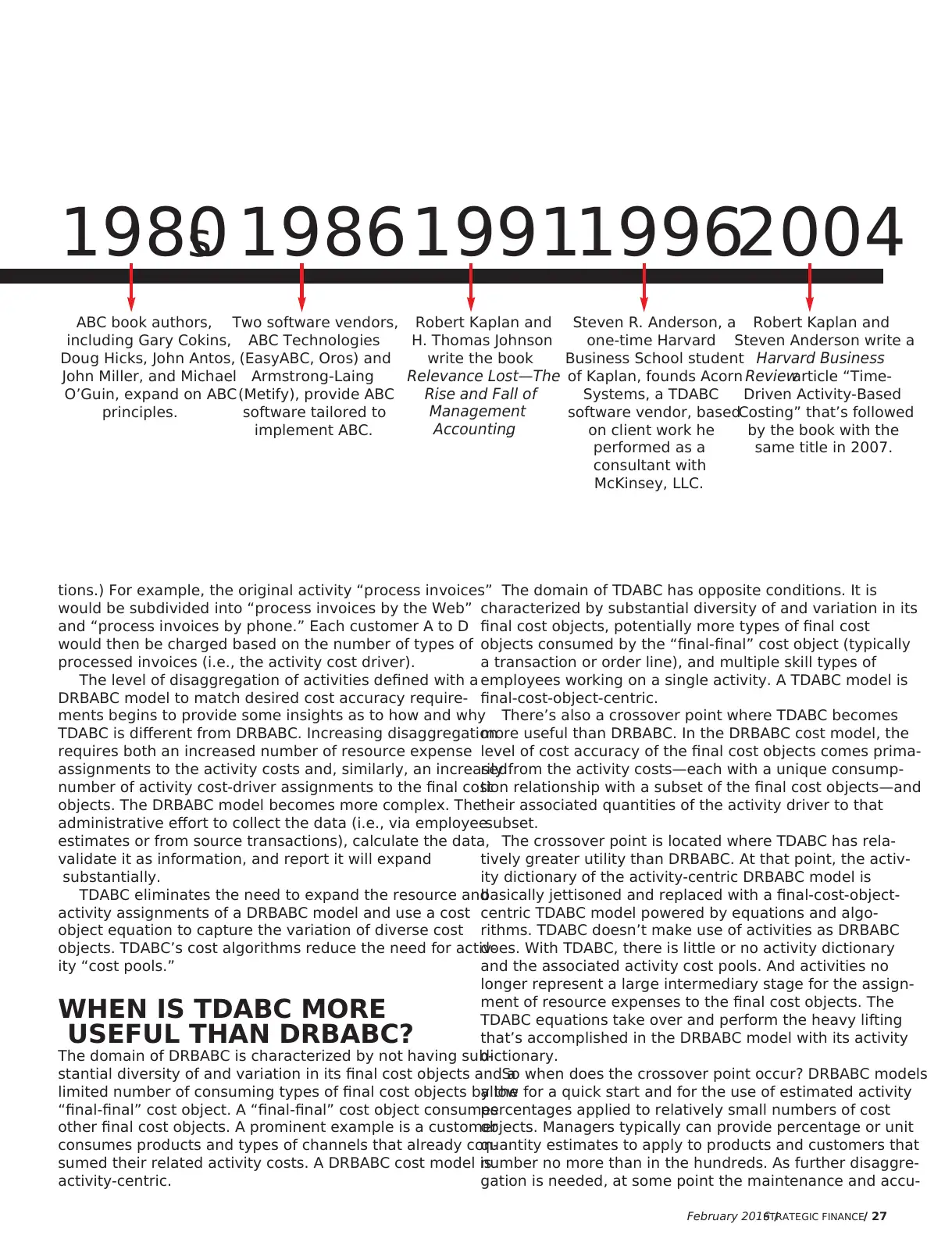
1980s
ABC book authors,
including Gary Cokins,
Doug Hicks, John Antos,
John Miller, and Michael
O’Guin, expand on ABC
principles.
1986
Two software vendors,
ABC Technologies
(EasyABC, Oros) and
Armstrong-Laing
(Metify), provide ABC
software tailored to
implement ABC.
1991
Robert Kaplan and
H. Thomas Johnson
write the book
Relevance Lost—The
Rise and Fall of
Management
Accounting.
1996
Steven R. Anderson, a
one-time Harvard
Business School student
of Kaplan, founds Acorn
Systems, a TDABC
software vendor, based
on client work he
performed as a
consultant with
McKinsey, LLC.
2004
Robert Kaplan and
Steven Anderson write a
Harvard Business
Reviewarticle “Time-
Driven Activity-Based
Costing” that’s followed
by the book with the
same title in 2007.
tions.) For example, the original activity “process invoices”
would be subdivided into “process invoices by the Web”
and “process invoices by phone.” Each customer A to D
would then be charged based on the number of types of
processed invoices (i.e., the activity cost driver).
The level of disaggregation of activities defined with a
DRBABC model to match desired cost accuracy require-
ments begins to provide some insights as to how and why
TDABC is different from DRBABC. Increasing disaggregation
requires both an increased number of resource expense
assignments to the activity costs and, similarly, an increased
number of activity cost-driver assignments to the final cost
objects. The DRBABC model becomes more complex. The
administrative effort to collect the data (i.e., via employee
estimates or from source transactions), calculate the data,
validate it as information, and report it will expand
substantially.
TDABC eliminates the need to expand the resource and
activity assignments of a DRBABC model and use a cost
object equation to capture the variation of diverse cost
objects. TDABC’s cost algorithms reduce the need for activ-
ity “cost pools.”
WHEN IS TDABC MORE
USEFUL THAN DRBABC?
The domain of DRBABC is characterized by not having sub-
stantial diversity of and variation in its final cost objects and a
limited number of consuming types of final cost objects by the
“final-final” cost object. A “final-final” cost object consumes
other final cost objects. A prominent example is a customer
consumes products and types of channels that already con-
sumed their related activity costs. A DRBABC cost model is
activity-centric.
The domain of TDABC has opposite conditions. It is
characterized by substantial diversity of and variation in its
final cost objects, potentially more types of final cost
objects consumed by the “final-final” cost object (typically
a transaction or order line), and multiple skill types of
employees working on a single activity. A TDABC model is
final-cost-object-centric.
There’s also a crossover point where TDABC becomes
more useful than DRBABC. In the DRBABC cost model, the
level of cost accuracy of the final cost objects comes prima-
rily from the activity costs—each with a unique consump-
tion relationship with a subset of the final cost objects—and
their associated quantities of the activity driver to that
subset.
The crossover point is located where TDABC has rela-
tively greater utility than DRBABC. At that point, the activ-
ity dictionary of the activity-centric DRBABC model is
basically jettisoned and replaced with a final-cost-object-
centric TDABC model powered by equations and algo-
rithms. TDABC doesn’t make use of activities as DRBABC
does. With TDABC, there is little or no activity dictionary
and the associated activity cost pools. And activities no
longer represent a large intermediary stage for the assign-
ment of resource expenses to the final cost objects. The
TDABC equations take over and perform the heavy lifting
that’s accomplished in the DRBABC model with its activity
dictionary.
So when does the crossover point occur? DRBABC models
allow for a quick start and for the use of estimated activity
percentages applied to relatively small numbers of cost
objects. Managers typically can provide percentage or unit
quantity estimates to apply to products and customers that
number no more than in the hundreds. As further disaggre-
gation is needed, at some point the maintenance and accu-
1980s
ABC book authors,
including Gary Cokins,
Doug Hicks, John Antos,
John Miller, and Michael
O’Guin, expand on ABC
principles.
1986
Two software vendors,
ABC Technologies
(EasyABC, Oros) and
Armstrong-Laing
(Metify), provide ABC
software tailored to
implement ABC.
1991
Robert Kaplan and
H. Thomas Johnson
write the book
Relevance Lost—The
Rise and Fall of
Management
Accounting.
1996
Steven R. Anderson, a
one-time Harvard
Business School student
of Kaplan, founds Acorn
Systems, a TDABC
software vendor, based
on client work he
performed as a
consultant with
McKinsey, LLC.
2004
Robert Kaplan and
Steven Anderson write a
Harvard Business
Reviewarticle “Time-
Driven Activity-Based
Costing” that’s followed
by the book with the
same title in 2007.
28 /STRATEGIC FINANCE/ February 2016
racy of a DRBABC model becomes stretched. The activity
dictionary grows and becomes more burdensome to
maintain.
At that point, the substitution of TDABC, with its more
data-driven approach and more transactional-level cost
object instances, becomes more suitable to the task and
easier to maintain. Organizations may not have all the
desirable driver data from their enterprise resource plan-
ning (ERP) systems for the time algorithms, but this
becomes less of a problem as software automation contin-
ues to improve. The added bonus is that TDABC provides
visibility to capacity utilization information while still pro-
viding full absorption of actual cost.
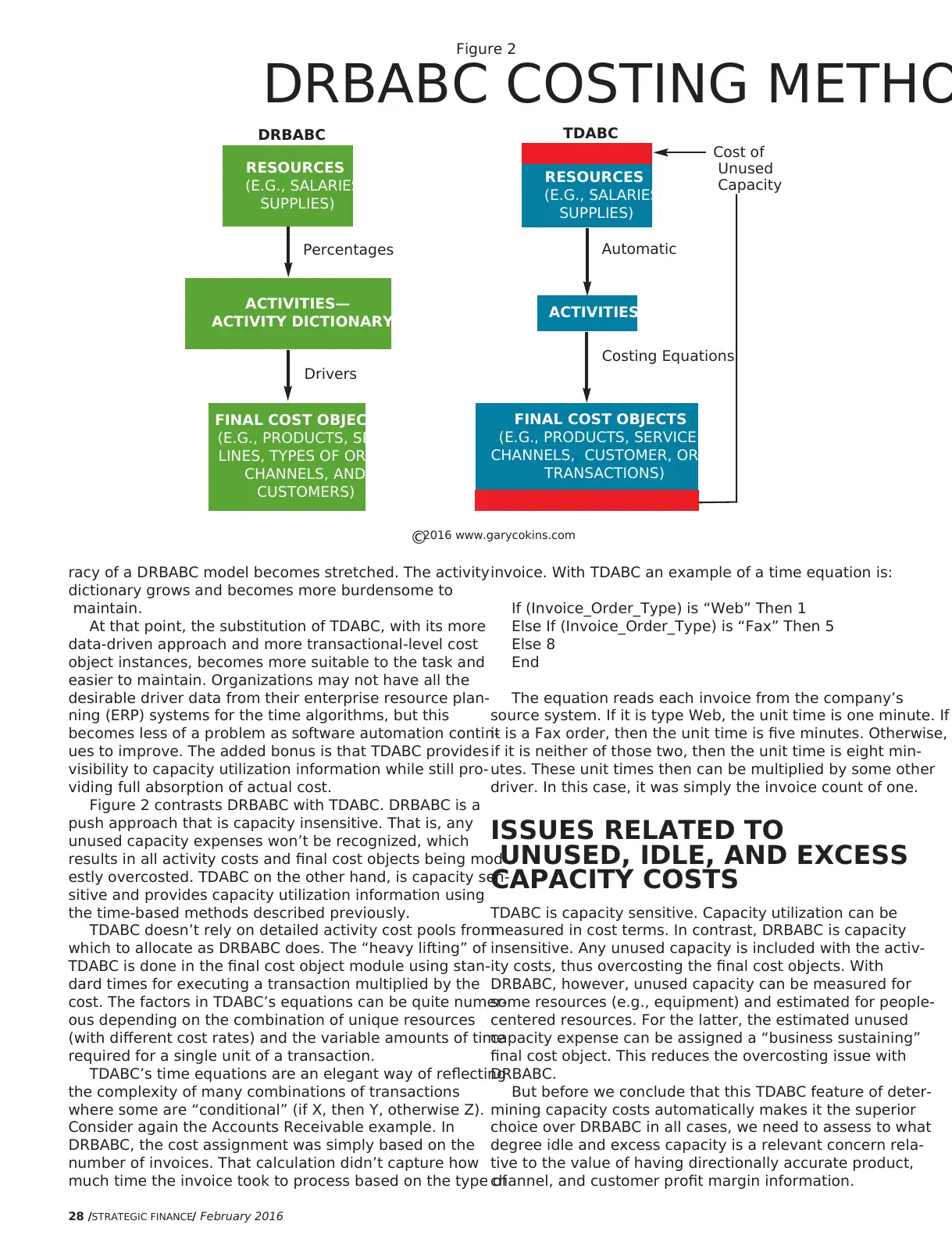
Figure 2 contrasts DRBABC with TDABC. DRBABC is a
push approach that is capacity insensitive. That is, any
unused capacity expenses won’t be recognized, which
results in all activity costs and final cost objects being mod-
estly overcosted. TDABC on the other hand, is capacity sen-
sitive and provides capacity utilization information using
the time-based methods described previously.
TDABC doesn’t rely on detailed activity cost pools from
which to allocate as DRBABC does. The “heavy lifting” of
TDABC is done in the final cost object module using stan-
dard times for executing a transaction multiplied by the
cost. The factors in TDABC’s equations can be quite numer-
ous depending on the combination of unique resources
(with different cost rates) and the variable amounts of time
required for a single unit of a transaction.
TDABC’s time equations are an elegant way of reflecting
the complexity of many combinations of transactions
where some are “conditional” (if X, then Y, otherwise Z).
Consider again the Accounts Receivable example. In
DRBABC, the cost assignment was simply based on the
number of invoices. That calculation didn’t capture how
much time the invoice took to process based on the type of
invoice. With TDABC an example of a time equation is:
If (Invoice_Order_Type) is “Web” Then 1
Else If (Invoice_Order_Type) is “Fax” Then 5
Else 8
End
The equation reads each invoice from the company’s
source system. If it is type Web, the unit time is one minute. If
it is a Fax order, then the unit time is five minutes. Otherwise,
if it is neither of those two, then the unit time is eight min-
utes. These unit times then can be multiplied by some other
driver. In this case, it was simply the invoice count of one.
ISSUES RELATED TO
UNUSED, IDLE, AND EXCESS
CAPACITY COSTS
TDABC is capacity sensitive. Capacity utilization can be
measured in cost terms. In contrast, DRBABC is capacity
insensitive. Any unused capacity is included with the activ-
ity costs, thus overcosting the final cost objects. With
DRBABC, however, unused capacity can be measured for
some resources (e.g., equipment) and estimated for people-
centered resources. For the latter, the estimated unused
capacity expense can be assigned a “business sustaining”
final cost object. This reduces the overcosting issue with
DRBABC.
But before we conclude that this TDABC feature of deter-
mining capacity costs automatically makes it the superior
choice over DRBABC in all cases, we need to assess to what
degree idle and excess capacity is a relevant concern rela-
tive to the value of having directionally accurate product,
channel, and customer profit margin information.
Figure 2
DRBABC COSTING METHO
RESOURCES
(E.G., SALARIES,
SUPPLIES)
RESOURCES
(E.G., SALARIES,
SUPPLIES)
ACTIVITIES—
ACTIVITY DICTIONARY ACTIVITIES
FINAL COST OBJECTS
(E.G., PRODUCTS, SERVICE
LINES, TYPES OF ORDERS,
CHANNELS, AND
CUSTOMERS)
FINAL COST OBJECTS
(E.G., PRODUCTS, SERVICE LINES,
CHANNELS, CUSTOMER, ORDER LINES,
TRANSACTIONS)
Cost of
Unused
Capacity
Percentages Automatic
Costing Equations
Drivers
©2016 www.garycokins.com
DRBABC TDABC
racy of a DRBABC model becomes stretched. The activity
dictionary grows and becomes more burdensome to
maintain.
At that point, the substitution of TDABC, with its more
data-driven approach and more transactional-level cost
object instances, becomes more suitable to the task and
easier to maintain. Organizations may not have all the
desirable driver data from their enterprise resource plan-
ning (ERP) systems for the time algorithms, but this
becomes less of a problem as software automation contin-
ues to improve. The added bonus is that TDABC provides
visibility to capacity utilization information while still pro-
viding full absorption of actual cost.
Figure 2 contrasts DRBABC with TDABC. DRBABC is a
push approach that is capacity insensitive. That is, any
unused capacity expenses won’t be recognized, which
results in all activity costs and final cost objects being mod-
estly overcosted. TDABC on the other hand, is capacity sen-
sitive and provides capacity utilization information using
the time-based methods described previously.
TDABC doesn’t rely on detailed activity cost pools from
which to allocate as DRBABC does. The “heavy lifting” of
TDABC is done in the final cost object module using stan-
dard times for executing a transaction multiplied by the
cost. The factors in TDABC’s equations can be quite numer-
ous depending on the combination of unique resources
(with different cost rates) and the variable amounts of time
required for a single unit of a transaction.
TDABC’s time equations are an elegant way of reflecting
the complexity of many combinations of transactions
where some are “conditional” (if X, then Y, otherwise Z).
Consider again the Accounts Receivable example. In
DRBABC, the cost assignment was simply based on the
number of invoices. That calculation didn’t capture how
much time the invoice took to process based on the type of
invoice. With TDABC an example of a time equation is:
If (Invoice_Order_Type) is “Web” Then 1
Else If (Invoice_Order_Type) is “Fax” Then 5
Else 8
End
The equation reads each invoice from the company’s
source system. If it is type Web, the unit time is one minute. If
it is a Fax order, then the unit time is five minutes. Otherwise,
if it is neither of those two, then the unit time is eight min-
utes. These unit times then can be multiplied by some other
driver. In this case, it was simply the invoice count of one.
ISSUES RELATED TO
UNUSED, IDLE, AND EXCESS
CAPACITY COSTS
TDABC is capacity sensitive. Capacity utilization can be
measured in cost terms. In contrast, DRBABC is capacity
insensitive. Any unused capacity is included with the activ-
ity costs, thus overcosting the final cost objects. With
DRBABC, however, unused capacity can be measured for
some resources (e.g., equipment) and estimated for people-
centered resources. For the latter, the estimated unused
capacity expense can be assigned a “business sustaining”
final cost object. This reduces the overcosting issue with
DRBABC.
But before we conclude that this TDABC feature of deter-
mining capacity costs automatically makes it the superior
choice over DRBABC in all cases, we need to assess to what
degree idle and excess capacity is a relevant concern rela-
tive to the value of having directionally accurate product,
channel, and customer profit margin information.
Figure 2
DRBABC COSTING METHO
RESOURCES
(E.G., SALARIES,
SUPPLIES)
RESOURCES
(E.G., SALARIES,
SUPPLIES)
ACTIVITIES—
ACTIVITY DICTIONARY ACTIVITIES
FINAL COST OBJECTS
(E.G., PRODUCTS, SERVICE
LINES, TYPES OF ORDERS,
CHANNELS, AND
CUSTOMERS)
FINAL COST OBJECTS
(E.G., PRODUCTS, SERVICE LINES,
CHANNELS, CUSTOMER, ORDER LINES,
TRANSACTIONS)
Cost of
Unused
Capacity
Percentages Automatic
Costing Equations
Drivers
©2016 www.garycokins.com
DRBABC TDABC
⊘ This is a preview!⊘
Do you want full access?
Subscribe today to unlock all pages.
Trusted by 1+ million students worldwide
February 2016 /STRATEGIC FINANCE/ 29
MAKING THE TRANSITION
As previously mentioned, whether a company selects
TDABC or DRBABC, the shared goal of both methods is to
move away from the single cost pool allocation factors that
violate costing’s causality principle. TDABC has advantages
with respect to level of detail, cost accuracy, automation,
and capacity calculation. But it also relies on capturing unit
times or other equation inputs for major business processes.
In many organizations, these simply aren’t available at the
onset of the initiative.
DRBABC has an advantage by enabling a quick start to
getting meaningful insight into costs and profitability.
Smaller activity lists and fewer numbers of final cost objects
that can be aggregated (e.g., product families, types of cus-
tomers) can be modeled quickly. Estimates from knowl-
edgeable cross-functional employees can be used initially
and iteratively be replaced with source data as needed. As
mentioned earlier, push cost assignments always normalize
to 100%. Understanding and needed buy-in from managers
for applying ABC can be achieved. Going forward in time,
the DRBABC model can also iteratively be disaggregated in
only selected parts of the model where further granularity
yields better or more accurate information. Once an organi-
zation matures and its informational needs become more
sophisticated, it can choose to migrate to TDABC.
We believe that all organizations can benefit from an
ABC cost assignment method and that either method dis-
cussed here is an improvement over what typically exists
with flawed and misleading cost and profit margin infor-
mation. For some organizations, starting with a DRBABC
model with subsequent iterative remodeling can be a fast
path toward results. Yet some organizations will, over time,
potentially reach the crossover point. From there onward,
TDABC offers increased benefits with regard to accuracy,
model maintenance, and overcoming the capacity-
insensitive nature of DRBABC.SF
Gary Cokins, CPIM, is IMA’s executive-in-residence and is founder
and owner of the consulting firm Analytics-Based Performance
Management LLC in Cary, N.C. (www.garycokins.com). A thought
leader in EPM, business analytics, and advanced cost management, he
previously was a consultant with Deloitte, KPMG, Electronic Data
Systems (EDS), and SAS. He also is a long-time member and active
committee member of IMA. You can reach Gary at (919) 720-2718 or
gcokins@garycokins.com.
Douglas D. Paul is solutions and engagement manager for Ignite
Technologies, formerly Acorn Systems, Inc. He has more than 25 years o
experience in finance software, consulting in cost and performance
management, and corporate positions in controllership and IT. You can
reach Doug at ddpaulpm@yahoo.com.
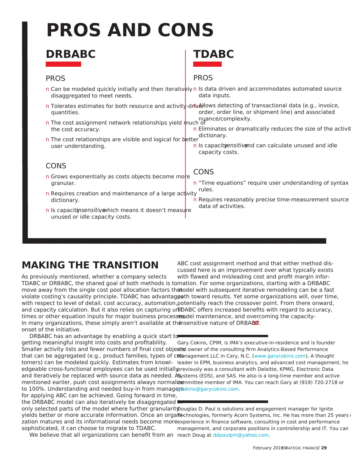
DRBABC
PROS
n Can be modeled quickly initially and then iteratively
disaggregated to meet needs.
n Tolerates estimates for both resource and activity-driver
quantities.
n The cost assignment network relationships yield much of
the cost accuracy.
n The cost relationships are visible and logical for better
user understanding.
CONS
n Grows exponentially as costs objects become more
granular.
n Requires creation and maintenance of a large activity
dictionary.
n Is capacityinsensitive, which means it doesn’t measure
unused or idle capacity costs.
TDABC
PROS
n Is data driven and accommodates automated source
data inputs.
n Allows detecting of transactional data (e.g., invoice,
order, order line, or shipment line) and associated
nuance/complexity.
n Eliminates or dramatically reduces the size of the activit
dictionary.
n Is capacitysensitiveand can calculate unused and idle
capacity costs.
CONS
n “Time equations” require user understanding of syntax
rules.
n Requires reasonably precise time-measurement source
data of activities.
PROS AND CONS
MAKING THE TRANSITION
As previously mentioned, whether a company selects
TDABC or DRBABC, the shared goal of both methods is to
move away from the single cost pool allocation factors that
violate costing’s causality principle. TDABC has advantages
with respect to level of detail, cost accuracy, automation,
and capacity calculation. But it also relies on capturing unit
times or other equation inputs for major business processes.
In many organizations, these simply aren’t available at the
onset of the initiative.
DRBABC has an advantage by enabling a quick start to
getting meaningful insight into costs and profitability.
Smaller activity lists and fewer numbers of final cost objects
that can be aggregated (e.g., product families, types of cus-
tomers) can be modeled quickly. Estimates from knowl-
edgeable cross-functional employees can be used initially
and iteratively be replaced with source data as needed. As
mentioned earlier, push cost assignments always normalize
to 100%. Understanding and needed buy-in from managers
for applying ABC can be achieved. Going forward in time,
the DRBABC model can also iteratively be disaggregated in
only selected parts of the model where further granularity
yields better or more accurate information. Once an organi-
zation matures and its informational needs become more
sophisticated, it can choose to migrate to TDABC.
We believe that all organizations can benefit from an
ABC cost assignment method and that either method dis-
cussed here is an improvement over what typically exists
with flawed and misleading cost and profit margin infor-
mation. For some organizations, starting with a DRBABC
model with subsequent iterative remodeling can be a fast
path toward results. Yet some organizations will, over time,
potentially reach the crossover point. From there onward,
TDABC offers increased benefits with regard to accuracy,
model maintenance, and overcoming the capacity-
insensitive nature of DRBABC.SF
Gary Cokins, CPIM, is IMA’s executive-in-residence and is founder
and owner of the consulting firm Analytics-Based Performance
Management LLC in Cary, N.C. (www.garycokins.com). A thought
leader in EPM, business analytics, and advanced cost management, he
previously was a consultant with Deloitte, KPMG, Electronic Data
Systems (EDS), and SAS. He also is a long-time member and active
committee member of IMA. You can reach Gary at (919) 720-2718 or
gcokins@garycokins.com.
Douglas D. Paul is solutions and engagement manager for Ignite
Technologies, formerly Acorn Systems, Inc. He has more than 25 years o
experience in finance software, consulting in cost and performance
management, and corporate positions in controllership and IT. You can
reach Doug at ddpaulpm@yahoo.com.
DRBABC
PROS
n Can be modeled quickly initially and then iteratively
disaggregated to meet needs.
n Tolerates estimates for both resource and activity-driver
quantities.
n The cost assignment network relationships yield much of
the cost accuracy.
n The cost relationships are visible and logical for better
user understanding.
CONS
n Grows exponentially as costs objects become more
granular.
n Requires creation and maintenance of a large activity
dictionary.
n Is capacityinsensitive, which means it doesn’t measure
unused or idle capacity costs.
TDABC
PROS
n Is data driven and accommodates automated source
data inputs.
n Allows detecting of transactional data (e.g., invoice,
order, order line, or shipment line) and associated
nuance/complexity.
n Eliminates or dramatically reduces the size of the activit
dictionary.
n Is capacitysensitiveand can calculate unused and idle
capacity costs.
CONS
n “Time equations” require user understanding of syntax
rules.
n Requires reasonably precise time-measurement source
data of activities.
PROS AND CONS
Paraphrase This Document
Need a fresh take? Get an instant paraphrase of this document with our AI Paraphraser

Reproduced with permission of the copyright owner. Further reproduction prohibited w
permission.
permission.
1 out of 11
Your All-in-One AI-Powered Toolkit for Academic Success.
+13062052269
info@desklib.com
Available 24*7 on WhatsApp / Email
![[object Object]](/_next/static/media/star-bottom.7253800d.svg)
Unlock your academic potential
Copyright © 2020–2026 A2Z Services. All Rights Reserved. Developed and managed by ZUCOL.