Econometric Analysis: VAR Model for Monetary Policy Transmission
VerifiedAdded on 2023/06/16
|11
|1401
|415
Report
AI Summary
This assignment focuses on analyzing the transmission mechanism of monetary policy using a Vector Autoregression (VAR) model. The analysis begins by identifying unit roots and stationary points using time series plots and Augmented Dickey-Fuller tests. The VAR model is constructed with a single lag, and three models are generated, including growth rate (GDP), inflation rate, and policy interest rate. The Engle-Granger method is then used to test for cointegration among the variables. The results indicate the presence of statistically significant factors in the monetary policy transmission mechanism, with both growth rate, inflation, and interest rates having statistically important negative and positive signs. The assignment concludes that the residuals are stationary, providing further evidence of cointegration due to the stationary process starting with non-stationary variables. Desklib offers a wealth of similar solved assignments and resources for students.

Running head: TIME SERIES ANALYSIS 1
Time Series Analysis
Name:
Institution:
Time Series Analysis
Name:
Institution:
Paraphrase This Document
Need a fresh take? Get an instant paraphrase of this document with our AI Paraphraser
TIME SERIES ANALYSIS 2
Time Series Analysis
Question 1
To test the VAR model, it is important to consider which variable needs to be considered for the
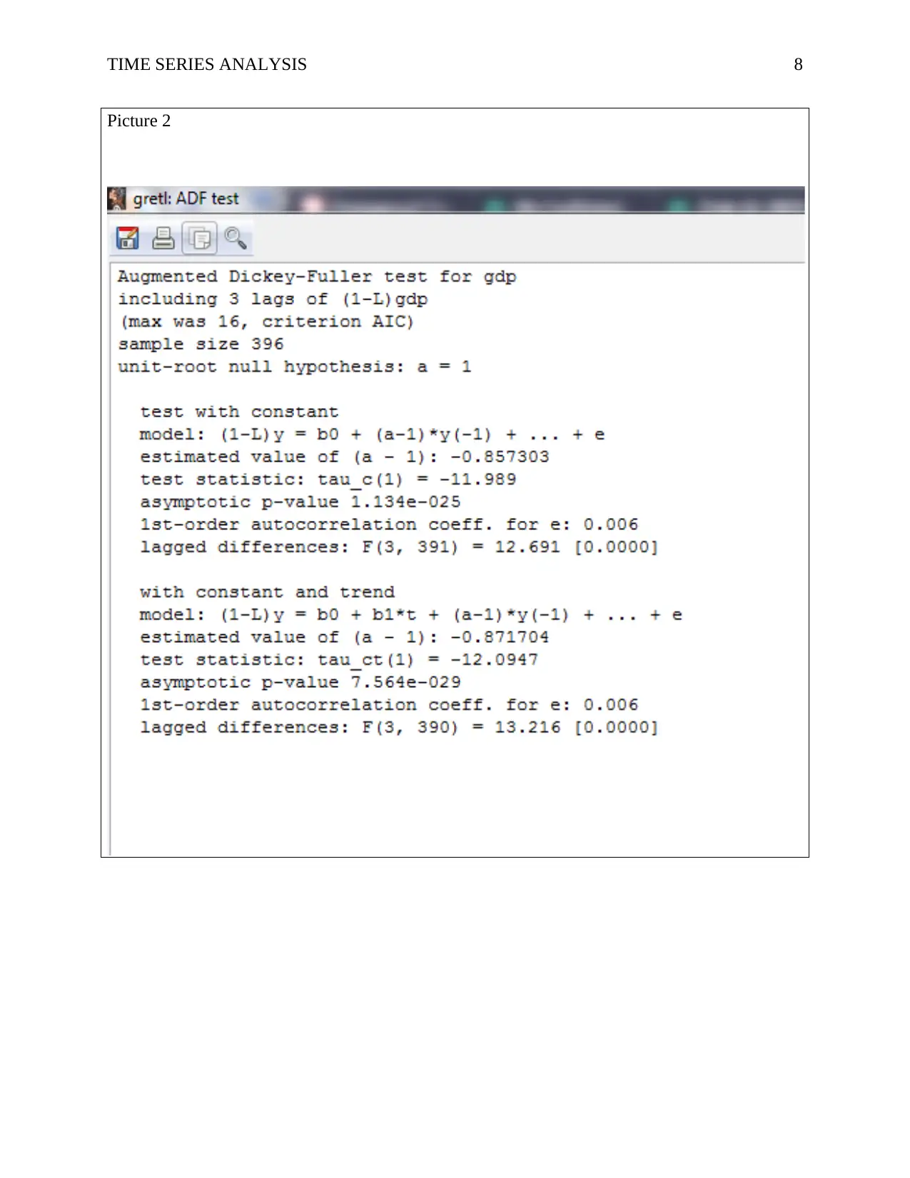
model. First, the unit root and stationary points must be identified. Then time series plots are
constructed in separate graphs as shown in picture 1to know if there is any trend or even a drift.
Having done the modeling of the transmission mechanism of the monetary policy as shown in
picture 1, it can be observed that there is no trend and that there is also no drift and also that the
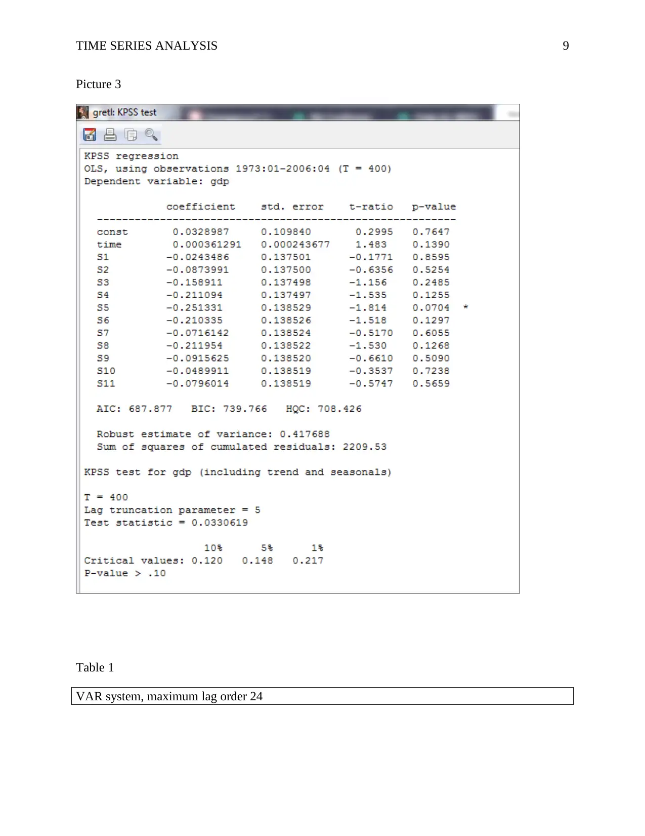
mean is around 0 (refer to picture 1). Next, an Augmented Dickey-Fuller test is performed in
efforts to identify the presence of unit root as shown in picture 2. Therefore, as seen in picture 2,
all the p-values move to zero (0); therefore, rejecting the null hypothesis in favor of the
alternative hypothesis which holds that there is unit root. Thus, there are three roots in the VAR
model. Furthermore, in order to clarify this, the KPSS test can be used to confirm as shown in
picture 3.
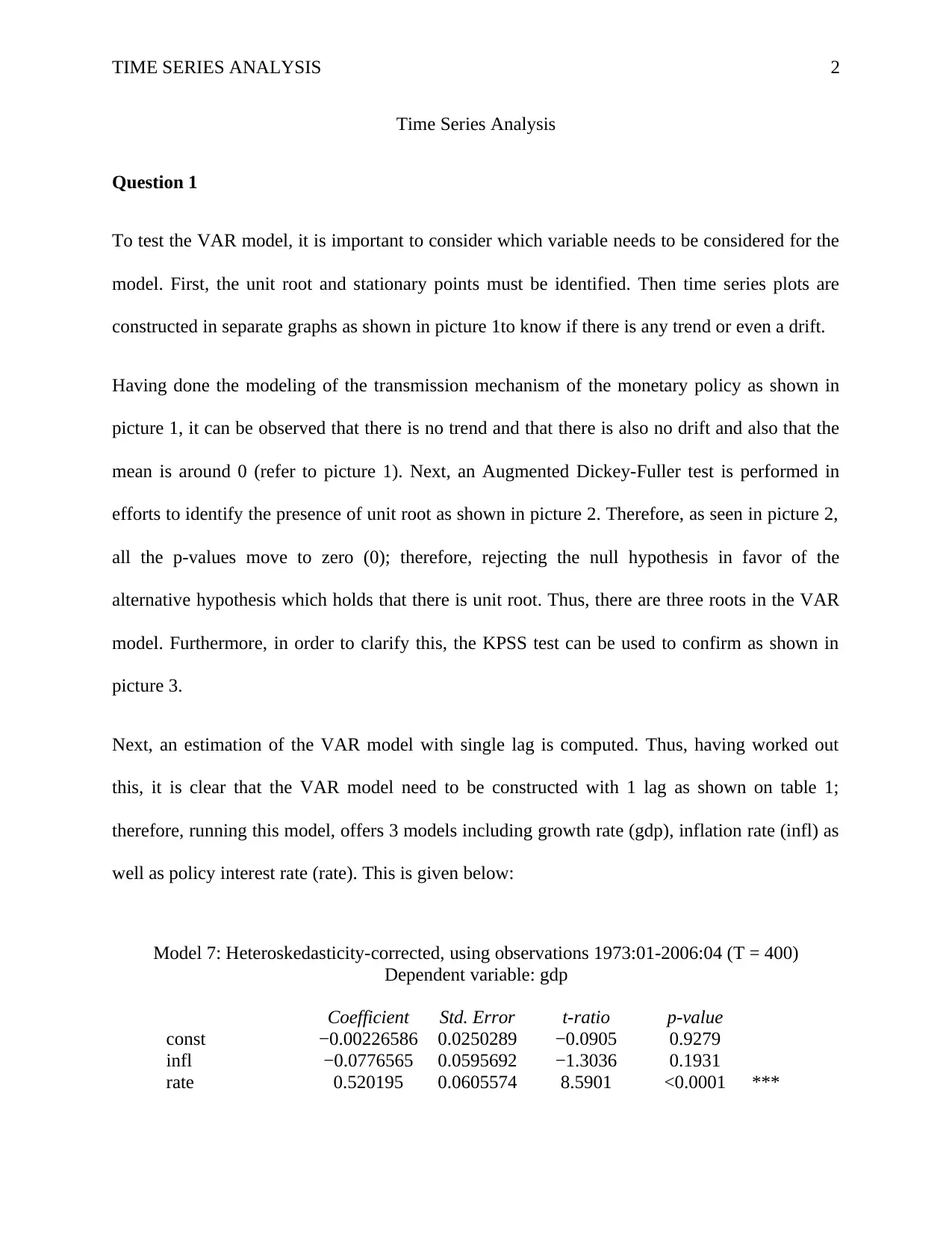
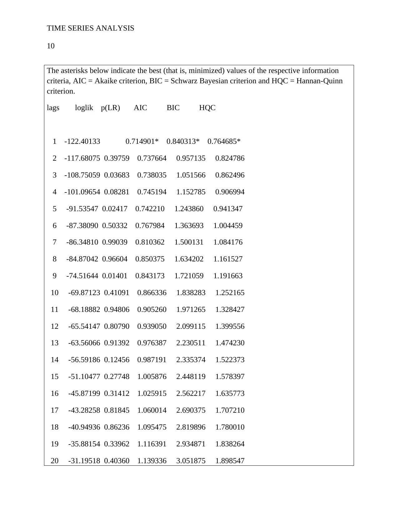
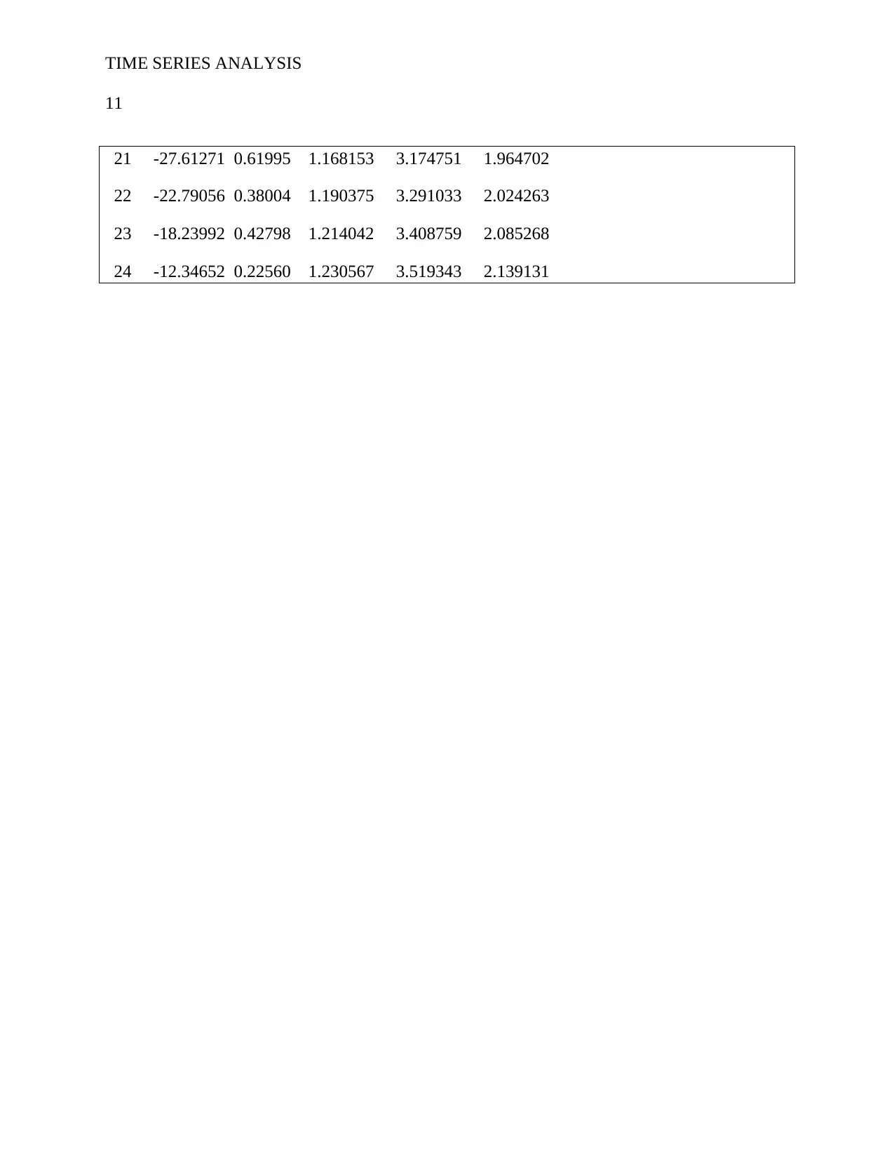
Next, an estimation of the VAR model with single lag is computed. Thus, having worked out
this, it is clear that the VAR model need to be constructed with 1 lag as shown on table 1;
therefore, running this model, offers 3 models including growth rate (gdp), inflation rate (infl) as
well as policy interest rate (rate). This is given below:
Model 7: Heteroskedasticity-corrected, using observations 1973:01-2006:04 (T = 400)
Dependent variable: gdp
Coefficient Std. Error t-ratio p-value
const −0.00226586 0.0250289 −0.0905 0.9279
infl −0.0776565 0.0595692 −1.3036 0.1931
rate 0.520195 0.0605574 8.5901 <0.0001 ***
TIME SERIES ANALYSIS 3
Statistics based on the weighted data:
Sum squared resid 1481.686 S.E. of regression 1.931892
R-squared 0.203055 Adjusted R-squared 0.199040
F(2, 397) 50.57601 P-value(F) 2.71e-20
Log-likelihood −829.4696 Akaike criterion 1664.939
Schwarz criterion 1676.914 Hannan-Quinn 1669.681
rho 0.481165 Durbin-Watson 1.037508
Statistics based on the original data:
Mean dependent var −0.015256 S.D. dependent var 0.561590
Sum squared resid 99.55367 S.E. of regression 0.500764
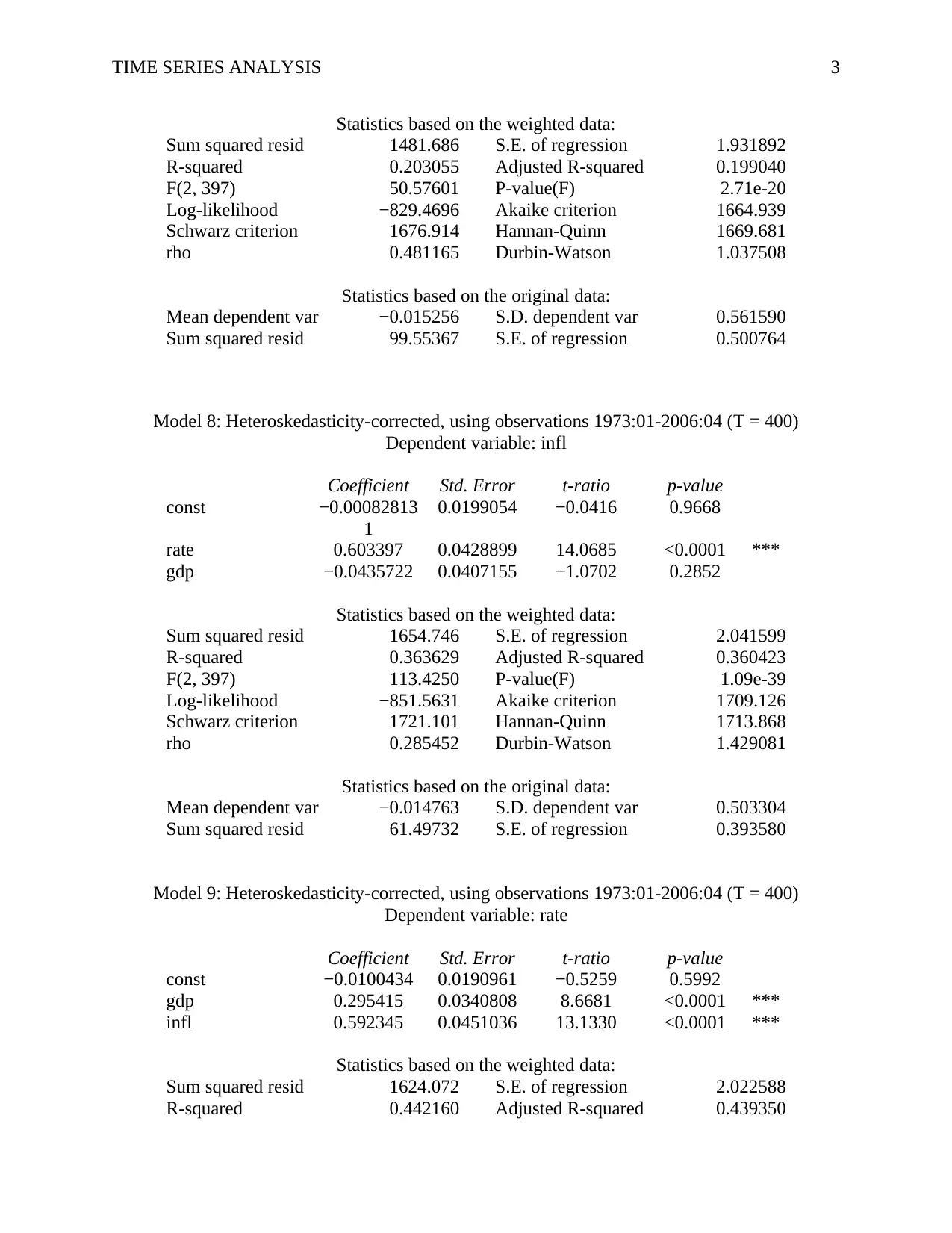
Model 8: Heteroskedasticity-corrected, using observations 1973:01-2006:04 (T = 400)
Dependent variable: infl
Coefficient Std. Error t-ratio p-value
const −0.00082813
1
0.0199054 −0.0416 0.9668
rate 0.603397 0.0428899 14.0685 <0.0001 ***
gdp −0.0435722 0.0407155 −1.0702 0.2852
Statistics based on the weighted data:
Sum squared resid 1654.746 S.E. of regression 2.041599
R-squared 0.363629 Adjusted R-squared 0.360423
F(2, 397) 113.4250 P-value(F) 1.09e-39
Log-likelihood −851.5631 Akaike criterion 1709.126
Schwarz criterion 1721.101 Hannan-Quinn 1713.868
rho 0.285452 Durbin-Watson 1.429081
Statistics based on the original data:
Mean dependent var −0.014763 S.D. dependent var 0.503304
Sum squared resid 61.49732 S.E. of regression 0.393580
Model 9: Heteroskedasticity-corrected, using observations 1973:01-2006:04 (T = 400)
Dependent variable: rate
Coefficient Std. Error t-ratio p-value
const −0.0100434 0.0190961 −0.5259 0.5992
gdp 0.295415 0.0340808 8.6681 <0.0001 ***
infl 0.592345 0.0451036 13.1330 <0.0001 ***
Statistics based on the weighted data:
Sum squared resid 1624.072 S.E. of regression 2.022588
R-squared 0.442160 Adjusted R-squared 0.439350
Statistics based on the weighted data:
Sum squared resid 1481.686 S.E. of regression 1.931892
R-squared 0.203055 Adjusted R-squared 0.199040
F(2, 397) 50.57601 P-value(F) 2.71e-20
Log-likelihood −829.4696 Akaike criterion 1664.939
Schwarz criterion 1676.914 Hannan-Quinn 1669.681
rho 0.481165 Durbin-Watson 1.037508
Statistics based on the original data:
Mean dependent var −0.015256 S.D. dependent var 0.561590
Sum squared resid 99.55367 S.E. of regression 0.500764
Model 8: Heteroskedasticity-corrected, using observations 1973:01-2006:04 (T = 400)
Dependent variable: infl
Coefficient Std. Error t-ratio p-value
const −0.00082813
1
0.0199054 −0.0416 0.9668
rate 0.603397 0.0428899 14.0685 <0.0001 ***
gdp −0.0435722 0.0407155 −1.0702 0.2852
Statistics based on the weighted data:
Sum squared resid 1654.746 S.E. of regression 2.041599
R-squared 0.363629 Adjusted R-squared 0.360423
F(2, 397) 113.4250 P-value(F) 1.09e-39
Log-likelihood −851.5631 Akaike criterion 1709.126
Schwarz criterion 1721.101 Hannan-Quinn 1713.868
rho 0.285452 Durbin-Watson 1.429081
Statistics based on the original data:
Mean dependent var −0.014763 S.D. dependent var 0.503304
Sum squared resid 61.49732 S.E. of regression 0.393580
Model 9: Heteroskedasticity-corrected, using observations 1973:01-2006:04 (T = 400)
Dependent variable: rate
Coefficient Std. Error t-ratio p-value
const −0.0100434 0.0190961 −0.5259 0.5992
gdp 0.295415 0.0340808 8.6681 <0.0001 ***
infl 0.592345 0.0451036 13.1330 <0.0001 ***
Statistics based on the weighted data:
Sum squared resid 1624.072 S.E. of regression 2.022588
R-squared 0.442160 Adjusted R-squared 0.439350
⊘ This is a preview!⊘
Do you want full access?
Subscribe today to unlock all pages.

Trusted by 1+ million students worldwide
TIME SERIES ANALYSIS 4
F(2, 397) 157.3367 P-value(F) 4.81e-51
Log-likelihood −847.8209 Akaike criterion 1701.642
Schwarz criterion 1713.616 Hannan-Quinn 1706.384
rho 0.507999 Durbin-Watson 0.984011
Statistics based on the original data:
Mean dependent var −0.024936 S.D. dependent var 0.535993
Sum squared resid 58.80561 S.E. of regression 0.384870
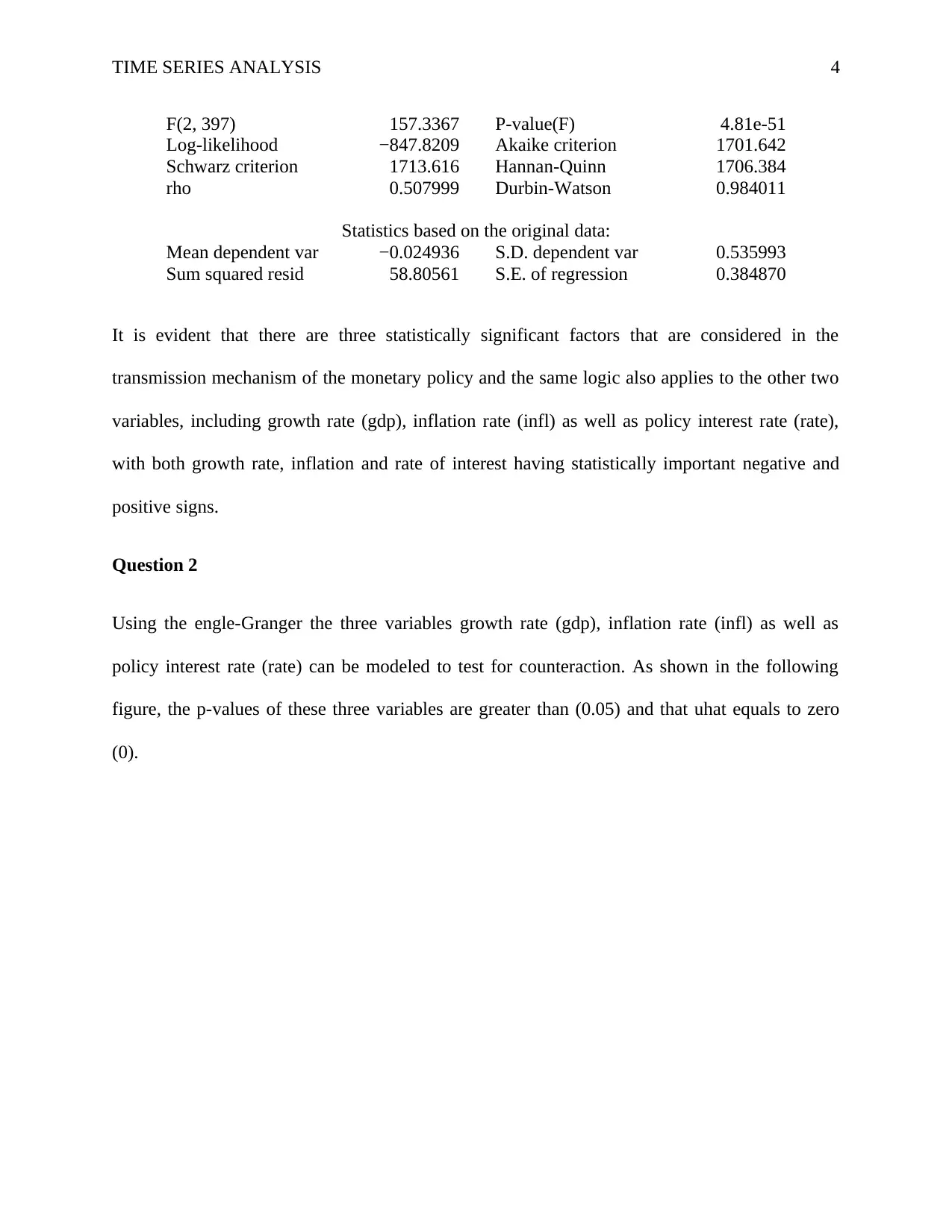
It is evident that there are three statistically significant factors that are considered in the
transmission mechanism of the monetary policy and the same logic also applies to the other two
variables, including growth rate (gdp), inflation rate (infl) as well as policy interest rate (rate),
with both growth rate, inflation and rate of interest having statistically important negative and
positive signs.
Question 2
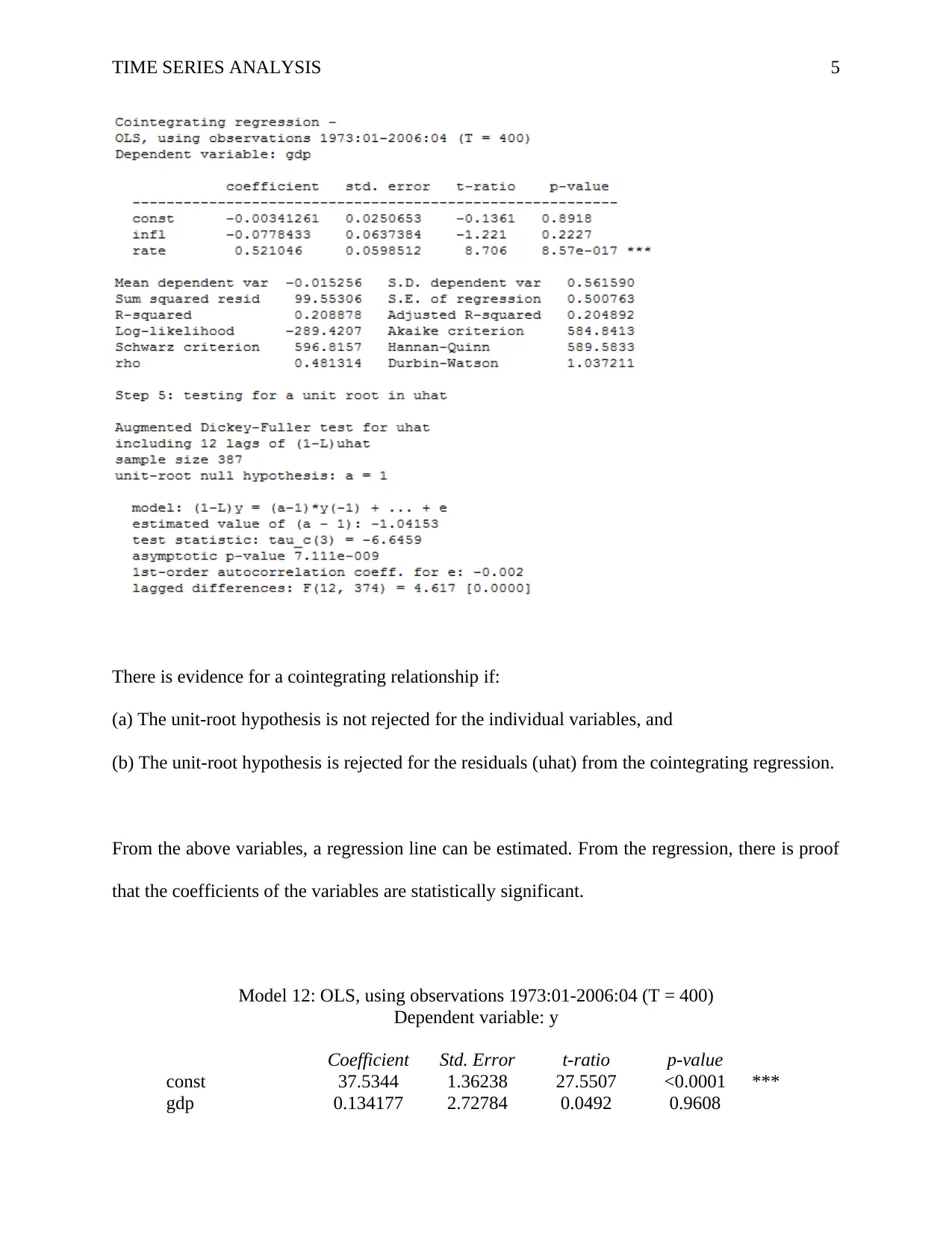
Using the engle-Granger the three variables growth rate (gdp), inflation rate (infl) as well as
policy interest rate (rate) can be modeled to test for counteraction. As shown in the following
figure, the p-values of these three variables are greater than (0.05) and that uhat equals to zero
(0).
Paraphrase This Document
Need a fresh take? Get an instant paraphrase of this document with our AI Paraphraser
TIME SERIES ANALYSIS 5
There is evidence for a cointegrating relationship if:
(a) The unit-root hypothesis is not rejected for the individual variables, and
(b) The unit-root hypothesis is rejected for the residuals (uhat) from the cointegrating regression.
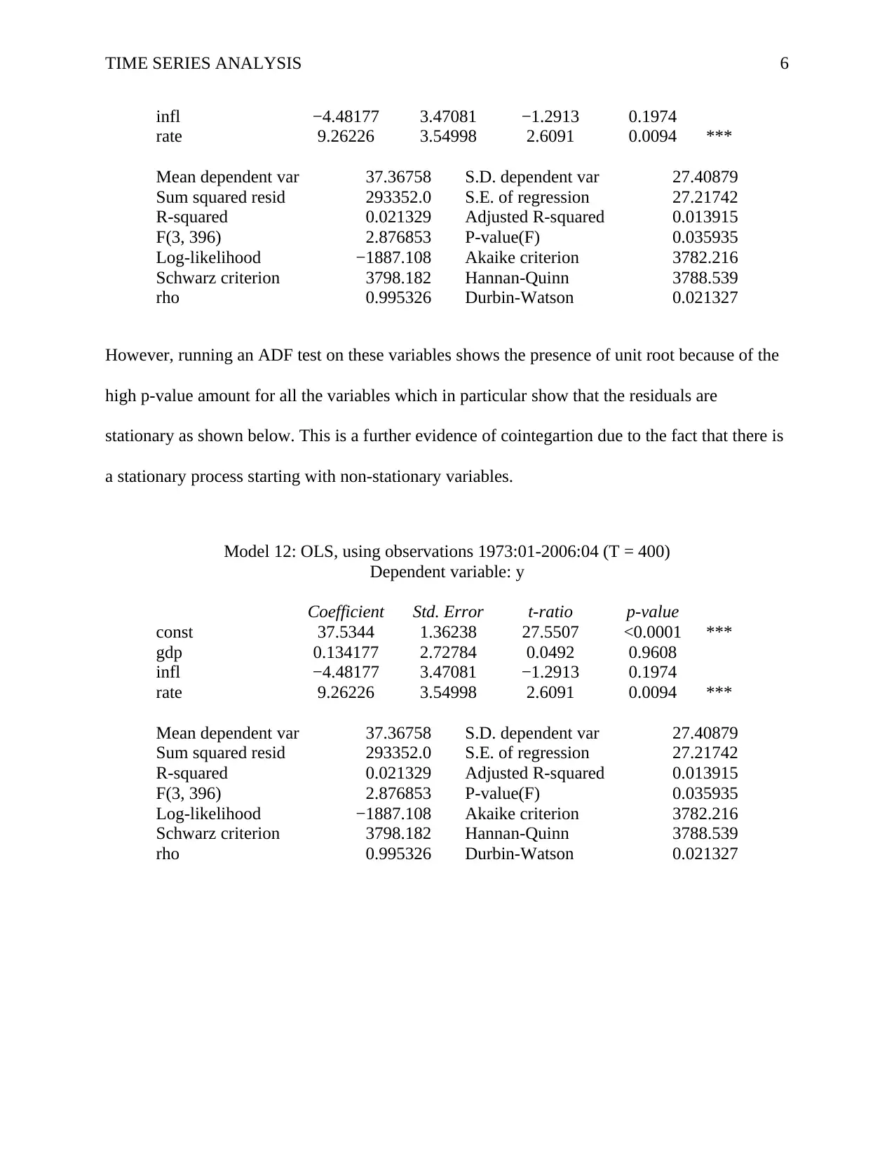
From the above variables, a regression line can be estimated. From the regression, there is proof
that the coefficients of the variables are statistically significant.
Model 12: OLS, using observations 1973:01-2006:04 (T = 400)
Dependent variable: y
Coefficient Std. Error t-ratio p-value
const 37.5344 1.36238 27.5507 <0.0001 ***
gdp 0.134177 2.72784 0.0492 0.9608
TIME SERIES ANALYSIS 6
infl −4.48177 3.47081 −1.2913 0.1974
rate 9.26226 3.54998 2.6091 0.0094 ***
Mean dependent var 37.36758 S.D. dependent var 27.40879
Sum squared resid 293352.0 S.E. of regression 27.21742
R-squared 0.021329 Adjusted R-squared 0.013915
F(3, 396) 2.876853 P-value(F) 0.035935
Log-likelihood −1887.108 Akaike criterion 3782.216
Schwarz criterion 3798.182 Hannan-Quinn 3788.539
rho 0.995326 Durbin-Watson 0.021327
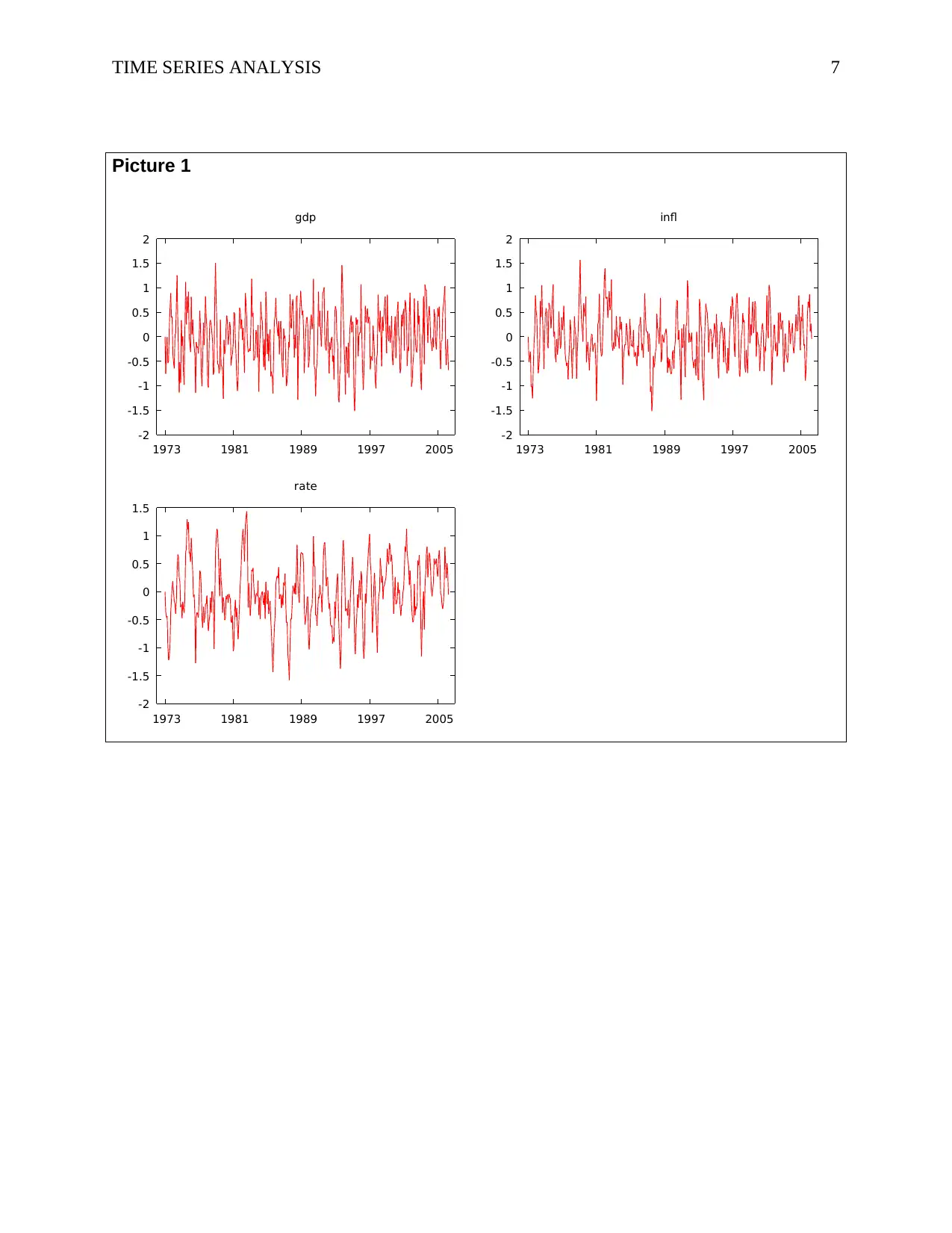
However, running an ADF test on these variables shows the presence of unit root because of the
high p-value amount for all the variables which in particular show that the residuals are
stationary as shown below. This is a further evidence of cointegartion due to the fact that there is
a stationary process starting with non-stationary variables.
Model 12: OLS, using observations 1973:01-2006:04 (T = 400)
Dependent variable: y
Coefficient Std. Error t-ratio p-value
const 37.5344 1.36238 27.5507 <0.0001 ***
gdp 0.134177 2.72784 0.0492 0.9608
infl −4.48177 3.47081 −1.2913 0.1974
rate 9.26226 3.54998 2.6091 0.0094 ***
Mean dependent var 37.36758 S.D. dependent var 27.40879
Sum squared resid 293352.0 S.E. of regression 27.21742
R-squared 0.021329 Adjusted R-squared 0.013915
F(3, 396) 2.876853 P-value(F) 0.035935
Log-likelihood −1887.108 Akaike criterion 3782.216
Schwarz criterion 3798.182 Hannan-Quinn 3788.539
rho 0.995326 Durbin-Watson 0.021327
However, running an ADF test on these variables shows the presence of unit root because of the
high p-value amount for all the variables which in particular show that the residuals are
stationary as shown below. This is a further evidence of cointegartion due to the fact that there is
a stationary process starting with non-stationary variables.
Model 12: OLS, using observations 1973:01-2006:04 (T = 400)
Dependent variable: y
Coefficient Std. Error t-ratio p-value
const 37.5344 1.36238 27.5507 <0.0001 ***
gdp 0.134177 2.72784 0.0492 0.9608
infl −4.48177 3.47081 −1.2913 0.1974
rate 9.26226 3.54998 2.6091 0.0094 ***
Mean dependent var 37.36758 S.D. dependent var 27.40879
Sum squared resid 293352.0 S.E. of regression 27.21742
R-squared 0.021329 Adjusted R-squared 0.013915
F(3, 396) 2.876853 P-value(F) 0.035935
Log-likelihood −1887.108 Akaike criterion 3782.216
Schwarz criterion 3798.182 Hannan-Quinn 3788.539
rho 0.995326 Durbin-Watson 0.021327
⊘ This is a preview!⊘
Do you want full access?
Subscribe today to unlock all pages.

Trusted by 1+ million students worldwide
TIME SERIES ANALYSIS 7
Picture 1
-2
-1.5
-1
-0.5
0
0.5
1
1.5
2
1973 1981 1989 1997 2005
gdp
-2
-1.5
-1
-0.5
0
0.5
1
1.5
2
1973 1981 1989 1997 2005
infl
-2
-1.5
-1
-0.5
0
0.5
1
1.5
1973 1981 1989 1997 2005
rate
Picture 1
-2
-1.5
-1
-0.5
0
0.5
1
1.5
2
1973 1981 1989 1997 2005
gdp
-2
-1.5
-1
-0.5
0
0.5
1
1.5
2
1973 1981 1989 1997 2005
infl
-2
-1.5
-1
-0.5
0
0.5
1
1.5
1973 1981 1989 1997 2005
rate
Paraphrase This Document
Need a fresh take? Get an instant paraphrase of this document with our AI Paraphraser
TIME SERIES ANALYSIS 8
Picture 2
Picture 2
TIME SERIES ANALYSIS 9
Picture 3
Table 1
VAR system, maximum lag order 24
Picture 3
Table 1
VAR system, maximum lag order 24
⊘ This is a preview!⊘
Do you want full access?
Subscribe today to unlock all pages.

Trusted by 1+ million students worldwide
TIME SERIES ANALYSIS
10
The asterisks below indicate the best (that is, minimized) values of the respective information
criteria, AIC = Akaike criterion, BIC = Schwarz Bayesian criterion and HQC = Hannan-Quinn
criterion.
lags loglik p(LR) AIC BIC HQC
1 -122.40133 0.714901* 0.840313* 0.764685*
2 -117.68075 0.39759 0.737664 0.957135 0.824786
3 -108.75059 0.03683 0.738035 1.051566 0.862496
4 -101.09654 0.08281 0.745194 1.152785 0.906994
5 -91.53547 0.02417 0.742210 1.243860 0.941347
6 -87.38090 0.50332 0.767984 1.363693 1.004459
7 -86.34810 0.99039 0.810362 1.500131 1.084176
8 -84.87042 0.96604 0.850375 1.634202 1.161527
9 -74.51644 0.01401 0.843173 1.721059 1.191663
10 -69.87123 0.41091 0.866336 1.838283 1.252165
11 -68.18882 0.94806 0.905260 1.971265 1.328427
12 -65.54147 0.80790 0.939050 2.099115 1.399556
13 -63.56066 0.91392 0.976387 2.230511 1.474230
14 -56.59186 0.12456 0.987191 2.335374 1.522373
15 -51.10477 0.27748 1.005876 2.448119 1.578397
16 -45.87199 0.31412 1.025915 2.562217 1.635773
17 -43.28258 0.81845 1.060014 2.690375 1.707210
18 -40.94936 0.86236 1.095475 2.819896 1.780010
19 -35.88154 0.33962 1.116391 2.934871 1.838264
20 -31.19518 0.40360 1.139336 3.051875 1.898547
Paraphrase This Document
Need a fresh take? Get an instant paraphrase of this document with our AI Paraphraser
TIME SERIES ANALYSIS
11
21 -27.61271 0.61995 1.168153 3.174751 1.964702
22 -22.79056 0.38004 1.190375 3.291033 2.024263
23 -18.23992 0.42798 1.214042 3.408759 2.085268
24 -12.34652 0.22560 1.230567 3.519343 2.139131
11
21 -27.61271 0.61995 1.168153 3.174751 1.964702
22 -22.79056 0.38004 1.190375 3.291033 2.024263
23 -18.23992 0.42798 1.214042 3.408759 2.085268
24 -12.34652 0.22560 1.230567 3.519343 2.139131
1 out of 11