Time Series Plots: Moving Average, Histograms, Kernel Density

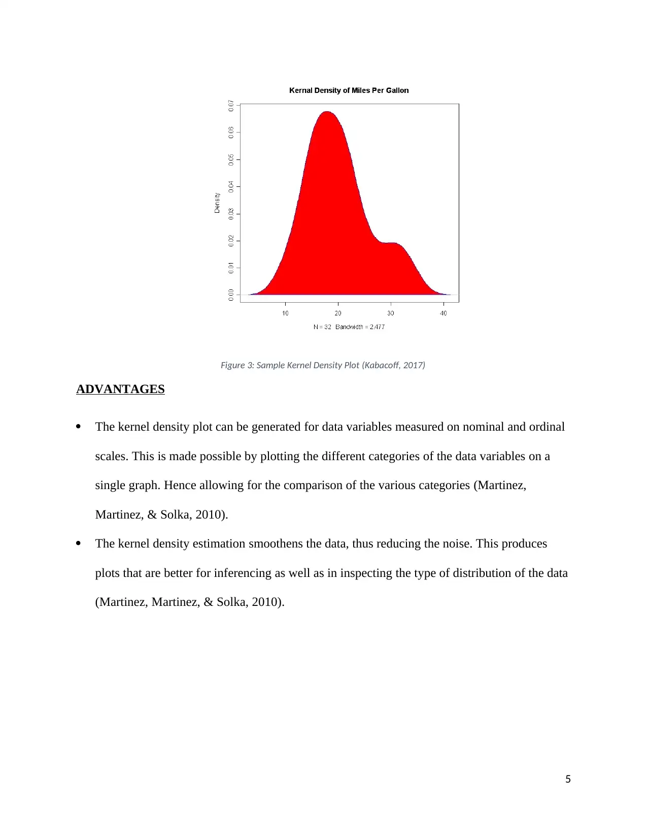
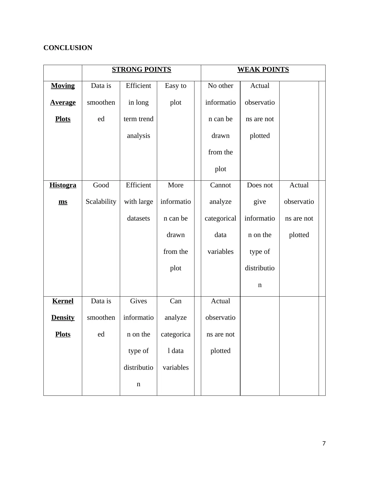
This report provides a comprehensive analysis of three key types of time series plots: moving average plots, histograms, and kernel density plots. It begins by defining each plot type and explaining its construction, including the use of moving averages to smooth data, the use of histograms to display the frequency of data variables, and the application of kernel density estimation. The report then delves into the advantages and disadvantages of each plot type, highlighting strengths such as the ease of generating moving average plots, the scalability of histograms, and the ability of kernel density plots to handle nominal and ordinal data. The report also discusses the limitations of each plot type, such as the inability of moving average plots to represent actual data observations, the lack of information on data distribution in histograms, and the fact that kernel density plots do not represent actual observations. The report concludes with a comparative summary, emphasizing the strong and weak points of each plot type, and provides relevant references to support the analysis.

1. MOVING AVERAGE PLOTS
This is a time series plot generated by separating the observations in the dataset into
subsets and obtaining the averages of the subsets (Hastie, Tibshir, & Jerome, 2009). These
averages are then plotted on a graph to produce the moving average plot. Since the plot largely
relies on the means, it is often also referred to as the Moving Means plot. This type of plot is
applied in the research on financial bubbles (Sam, David, Leybourne, Robert, & Taylor, 2018).
Figure 1: Sample Moving Average Plot (Sam, David, Leybourne, Robert, & Taylor, 2018)
ADVANTAGES
 The moving average plot is fairly an easy plot to construct. This is especially true for the
manual plotting of the observations. Instead of plotting the entire observations in the dataset,
the dataset is divided into subsets of n observations. This produces fewer points for plotting.
(Hastie, Tibshir, & Jerome, 2009)
 The moving average plot is efficient in generating the long term trends for the data. This plot
for the time series is appropriate for cases where data has been collected over long periods.
(Hastie, Tibshir, & Jerome, 2009)
 This plot smoothens the observations of the dataset. (Hastie, Tibshir, & Jerome, 2009)
1

DISADVANTAGES
 The moving average plot uses means, this makes it inefficient at identifying other properties
of a dataset. These properties, such as the outlier observations, would not be noticed since the
averaging tends to hide the extreme observations (Hastie, Tibshir, & Jerome, 2009).
 The moving average plot is not appropriate for generating the short term trends (Hastie,
Tibshir, & Jerome, 2009).
 With the use of the means, the moving average plot does not represent the actual data
observations (Hastie, Tibshir, & Jerome, 2009).
2. HISTOGRAMS
These are time series graphs that plot the frequencies of a variable in a dataset by
dividing the variable into intervals (Barbara & Susan, 2014). The time series analysis in the case
of the histogram involves simplification of the observations of the data variable. This is done by
introducing intervals of a predetermined and normally equal lengths. These intervals are then
plotted to produce the histogram. Histograms are used to describe the trend in the time series for
the oil and gas reservoirs (Hodaway, Fabii, & Lozie, 2015).
2

Figure 2: Sample Histogram Plot (Kabacoff, 2017)
ADVANTAGES
 The histogram can comfortably handle large datasets without its quality being affected. This
is the scalability characteristic of the histogram. This makes the varying of the size of data
being plotted (at least in an incremental sense) possible without compromising the quality of
the histogram produced (Barbara & Susan, 2014).
 In instances where the dataset being analyzed is significantly large (big data), the histogram
proves to be the most efficient plotting tool for the trend. The histogram gives better
visualization of the trend compared to other plotting tools for time series (Barbara & Susan,
2014).
 The histograms provide more information about the observations in the dataset other than the
trend. The statistics of the observations that can be derived from the histogram are outlier,
abnormality, skewness, centrality and spread (Barbara & Susan, 2014).
DISADVANTAGES
3

 Similar to the moving average plot, the histogram cannot be said to represent the actual data
observations. This is since the frequency of the observations themselves are not plotted, but
rather the frequency of the intervals (Barbara & Susan, 2014).
 The histogram cannot give information on the type of distribution of the data (Barbara &
Susan, 2014).
 The histogram, unlike the bar graph, is limited to giving the frequency information for the
non-categorical data variables. In cases the data variables are measured on the nominal or
ordinal scale (hence categorical), the histogram cannot be plotted. This narrows the
applications of the histograms to a large extent (Barbara & Susan, 2014).
3. KERNEL DENSITY PLOTS
These graphs use the kernel density estimation as a basis for generating the plots for the
time series (Martinez, Martinez, & Solka, 2010). The kernel density plots were used in testing
whether financial returns exhibit predictability (Imanol & Ignacio, 2015).
4

Figure 3: Sample Kernel Density Plot (Kabacoff, 2017)
ADVANTAGES
 The kernel density plot can be generated for data variables measured on nominal and ordinal
scales. This is made possible by plotting the different categories of the data variables on a
single graph. Hence allowing for the comparison of the various categories (Martinez,
Martinez, & Solka, 2010).
 The kernel density estimation smoothens the data, thus reducing the noise. This produces
plots that are better for inferencing as well as in inspecting the type of distribution of the data
(Martinez, Martinez, & Solka, 2010).
5

DISADVANTAGES
 The application of the kernel density estimation process implies that the actual observations
are not represented in the plot (Martinez, Martinez, & Solka, 2010).
6

CONCLUSION
STRONG POINTS WEAK POINTS
Moving
Average
Plots
Data is
smoothen
ed
Efficient
in long
term trend
analysis
Easy to
plot
No other
informatio
n can be
drawn
from the
plot
Actual
observatio
ns are not
plotted
Histogra
ms
Good
Scalability
Efficient
with large
datasets
More
informatio
n can be
drawn
from the
plot
Cannot
analyze
categorical
data
variables
Does not
give
informatio
n on the
type of
distributio
n
Actual
observatio
ns are not
plotted
Kernel
Density
Plots
Data is
smoothen
ed
Gives
informatio
n on the
type of
distributio
n
Can
analyze
categorica
l data
variables
Actual
observatio
ns are not
plotted
7

References
Barbara, I., & Susan, D. (2014). Introductory Statistics (1st ed.). New York: OpenStax CNX.
Hastie, T., Tibshir, R., & Jerome, H. (2009). The Elements of Statistical Learning (2nd ed.). New
York: Springer.
Hodaway, K. R., Fabii, L., & Lozie, D. (2015). Unconventional Data-Driven Methodologies
Forecast Performance in Unconventional Oil and Gas Reservoirs. SAS Istitutue, Inc, 1-12.
Imanol, A., & Ignacio, N. L. (2015). Testing for Predictability in Financial Returns Using
Statistical Learning Procedures. Journal of Time Series Analysis, 36(5). 1-13.
Kabacoff, R. I. (2017, March 15). graphs. Retrieved from statmethods:
www.statmethods.net/graphs/density.html
Martinez, W. L., Martinez, A. R., & Solka, J. (2010). Exploratory Data Analysis With MATLAB,
2nd Edition (1 ed.). London: CRC/Chapmann & Hall.
Sam, A., David, I. H., Leybourne, S. J., Robert, S., & Taylor, A. M. (2018). Real Time
Monitoring for Explosive Financial Bubbles. Journal of Time Series Analysis, 39(8) 1-7.
8