Numerical Integration Methods

The assignment focuses on numerical integration techniques used to approximate the area under a curve. It delves into two specific methods: Simpson's Rule and the Trapezium Rule. Simpson's Rule utilizes quadratic approximations, while the Trapezium Rule employs trapezoidal shapes to estimate the integral. The document illustrates how these methods work, providing examples and calculations.

Q.No:1
(A)
The transfer function provides a basis for determining important system response
characteristics
without solving the complete differential equation. As defined, the transfer function is a
rational
function in the complex variable s = σ + jω, that is
H(s) = bmsm + bm−1sm−1 + ... + b1s + b0
ansn + an−1sn−1 + ... + a1s + a0
(1)
It is often convenient to factor the polynomials in the numerator and denominator, and to write
the transfer function in terms of those factors:
H(s) = N(s)
D(s) = K (s − z1)(s − z2)...(s − zm−1)(s − zm)
(s − p1)(s − p2)...(s − pn−1)(s − pn)
, (2)
where the numerator and denominator polynomials, N(s) and D(s), have real coefficients
defined
by the system’s differential equation and K = bm/an. As written in Eq. (2) the zi’s are the roots
of the equation
N(s)=0, (3)
and are defined to be the system zeros, and the pi’s are the roots of the equation
D(s)=0, (4)
and are defined to be the system poles. In Eq. (2) the factors in the numerator and
denominator
are written so that when s = zi the numerator N(s) = 0 and the transfer function vanishes, that is

lims→zi
H(s)=0.
and similarly when s = pi the denominator polynomial D(s) = 0 and the value of the transfer
function becomes unbounded,
lims→pi
H(s) = ∞.
All of the coefficients of polynomials N(s) and D(s) are real, therefore the poles and zeros must
be either purely real, or appear in complex conjugate pairs. In general for the poles, either pi =
σi,
or else pi, pi+1 = σi±jωi. The existence of a single complex pole without a corresponding
conjugate
pole would generate complex coefficients in the polynomial D(s). Similarly, the system zeros are
either real or appear in complex conjugate pairs.
(B)
(i)
We wish to know if a system with transfer function
G(s) = 1 s + γ is stable. If γ < 0, let u(t)
= σ(t), the unit step function, which is obviously bounded.
Then, y(t) = L −1 [ 1 s (s + γ) ] = L −1 [ 1 γ ( 1 s − 1 s + γ )]
= 1 γ (1 − e −γt)σ(t), which goes to ∞ when t goes to ∞,
and hence is unbounded. This shows that the system is unstable.
If
γ = 0,
the system is called an integrator. Again let u(t)
= σ(t). Then, y(t) = L −1 [ 1 s 2 ]
= tσ(t), which goes to ∞ as t goes to ∞.
This shows that the system is again unstable.

If γ > 0, the impulse response of G(s) is g(t)
= e −γtσ(t). Then, |y(t)|
= ∫ t 0 g(τ )u(t − τ )dτ ≤ ∫ t 0 |g(τ )||u(t − τ )|dτ. If |u(t)| ≤ M for all t ∈ [0, ∞),
then |y(t)| ≤ M ∫ ∞ 0 |g(τ )|dτ
= M ∫ ∞ 0 e −γτ dτ
= M γ . Hence, as long as u(t) is bounded by M, then y(t) is bounded by M/γ. This shows that the system
is stable. In summary, a system with transfer function G(s)
= 1 s + γ is stable if γ > 0 and is unstable if γ ≤ 0.
Using the procedure in the example to test the stability of a system is often tedious. We desire to have
a simple stability test.
An LTI system with impulse response function g(t) is stable if and only if ∫ ∞ 0 |g(t)|dt < ∞. (3.1) Proof .
Assume that the input u(t) is bounded by M; then |y(t)|
= ∫ t 0 g(τ )u(t − τ )dτ
≤ ∫ t 0 |g(τ )||u(t − τ )|dτ ≤ M ∫ ∞ 0 |g(τ )|dτ.
Stability and Stabilization If (3.1) is satisfied, choose N = M ∫ ∞ 0 |g(τ )|dτ , and then the input bounded
by M generates the output bounded by N; i.e.,
the system is stable. This shows the sufficiency. If (3.1) is not satisfied,
∫ ∞ 0 |g(t)|dt = ∞. For any M > 0, choose t0 so that ∫ t0 0 |g(τ )|dτ > M and choose u(t)
= { 1, if g(t0 − t) ≥ 0; −1, if g(t0 − t) < 0 for 0 ≤ t ≤ t0. Then, |y(t0)|
= ∫ t0 0 g(t0 − τ )u(τ )dτ
= ∫ t0 0 |g(t0 − τ )|dτ
= ∫ t0 0 |g(τ )|dτ > M.
This shows that for an input u(t) bounded by 1, the output can be arbitrarily large. Hence, the system is
not stable. This proves the necessity. A signal is said to be absolutely integrable over an interval if the
integral of the absolute value of the signal over the interval is finite. Hence, a linear system is stable if its
impulse response is absolutely integrable over [0, ∞). This theorem makes it a bit easier to check the
stability of a system.
(ii)
Defining the function F and a subset of its domain : pts :
F[z_] := (5 - I z)/(5^2 + z^2)
pts = {-7, -2, 0, 2, 7};
the most straightforward way fulfilling the task is based on ParametricPlot and Epilog. We
can also make a diagram with the basic graphics primitives like e.g. : Line, Circle, Point.
Here are the both ways enclosed in GraphicsRow :

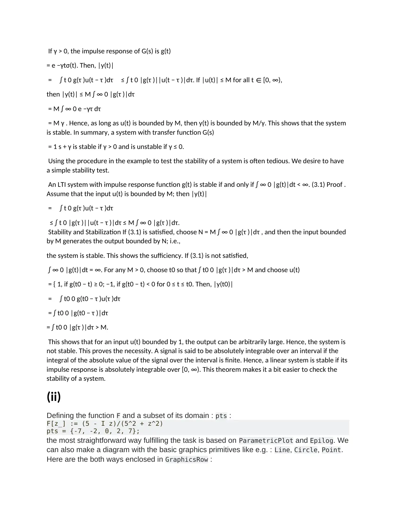
GraphicsRow[{
Graphics[{Line[{{0, -0.1}, {0, 0.1}}], Line[{{0, 0}, {0.21, 0}}],
Blue, Thick, Circle[{0.1, 0}, 0.1],
Red, PointSize[.03], Point[{Re @ #, Im @ #} & /@ F[pts]]}],
ParametricPlot[{Re @ #, Im @ #}& @ F[z], {z, -200, 200}, PlotRange ->
All,
PlotStyle -> Thick, Epilog -> { Red, PointSize[0.03],
Point[{Re @ F @ #, Im @ F @ #} & /@ pts]}] }]
Studying properties of holomorphic complex mappings is really rewarding, therefore one
should take a closer look at it. This function has a simple pole in 5 I :
Residue[ F[z], {z, 5 I}]
-I
and it is conformal in its domain :
Reduce[ D[ F[z], z] == 0, z]
False
i.e. it preserves angles locally. One can easily recognize the type of F evaluating Simplify[
F[z]], namely it is a composition of a translation, rescaling and inversion. We should look
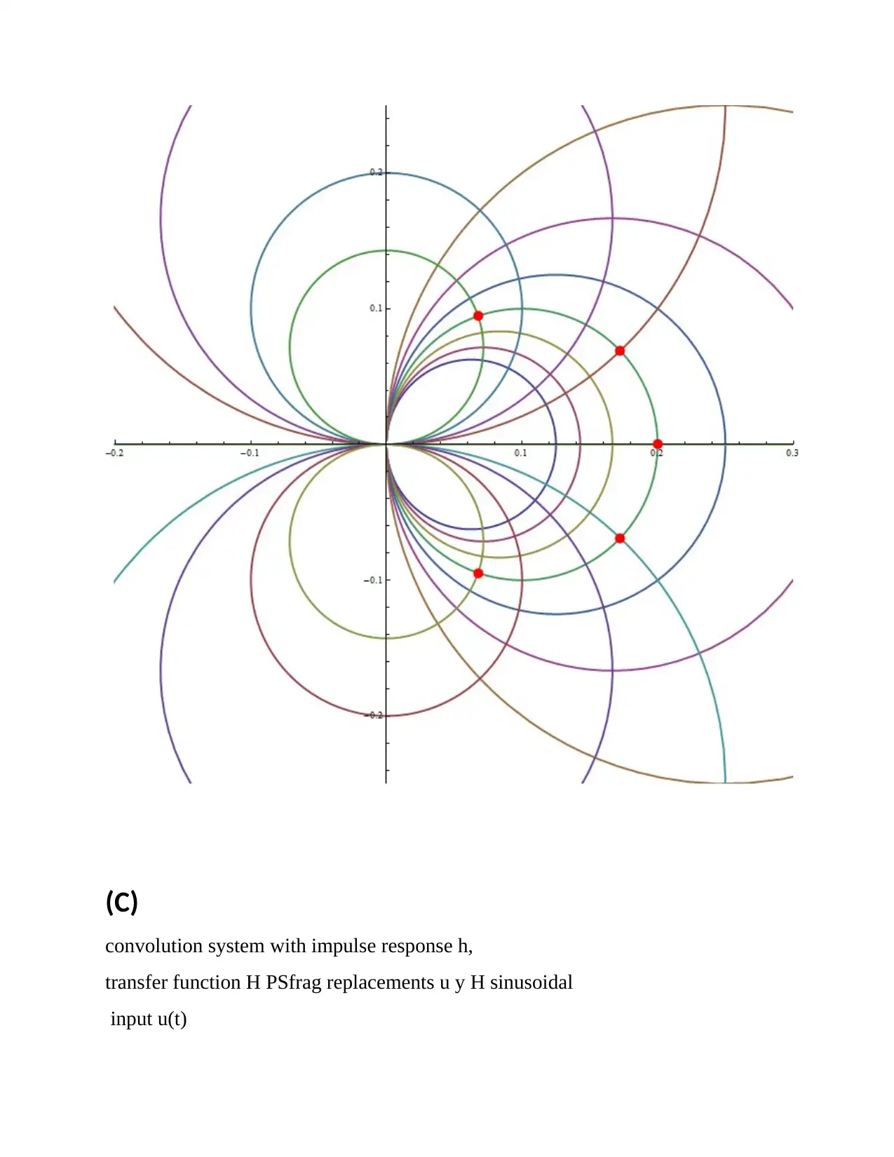
at images (via F) of simple geometric objects. To visualize the structure of the mapping F we
choose an appropriate grid in the complex domain of F and look at its image. We take a
continuous parameter $t$ varying in a range $(-25, 25)$ and contours $\;t+ i\;y $ for $y$ in a
discrete set of values $\{-3, -2,-1, 0, 1, 2, 3 \}$ and another orthogonal contours $\;x+ i\;t$
for $x$ in a discrete set $\{-7,-5,-3, -2, 0, 2, 3, 5, 5\;\}$, i.e.we have a grid of straight lines in
the complex plane. Next we'd like to plot the image of this grid through the mapping $F$.
Images of every line in the grid will be circles with centers on the abscissa and ordinate
respectively intersecting orthogonally. The red points denote values of $F(x)$ on the
complex plane for $x$ in $\{-7, -2, 0, 2, 7 \}$. On the lhs we have the original grid in the
domain of Fand on the rhs we have the plot of its image :

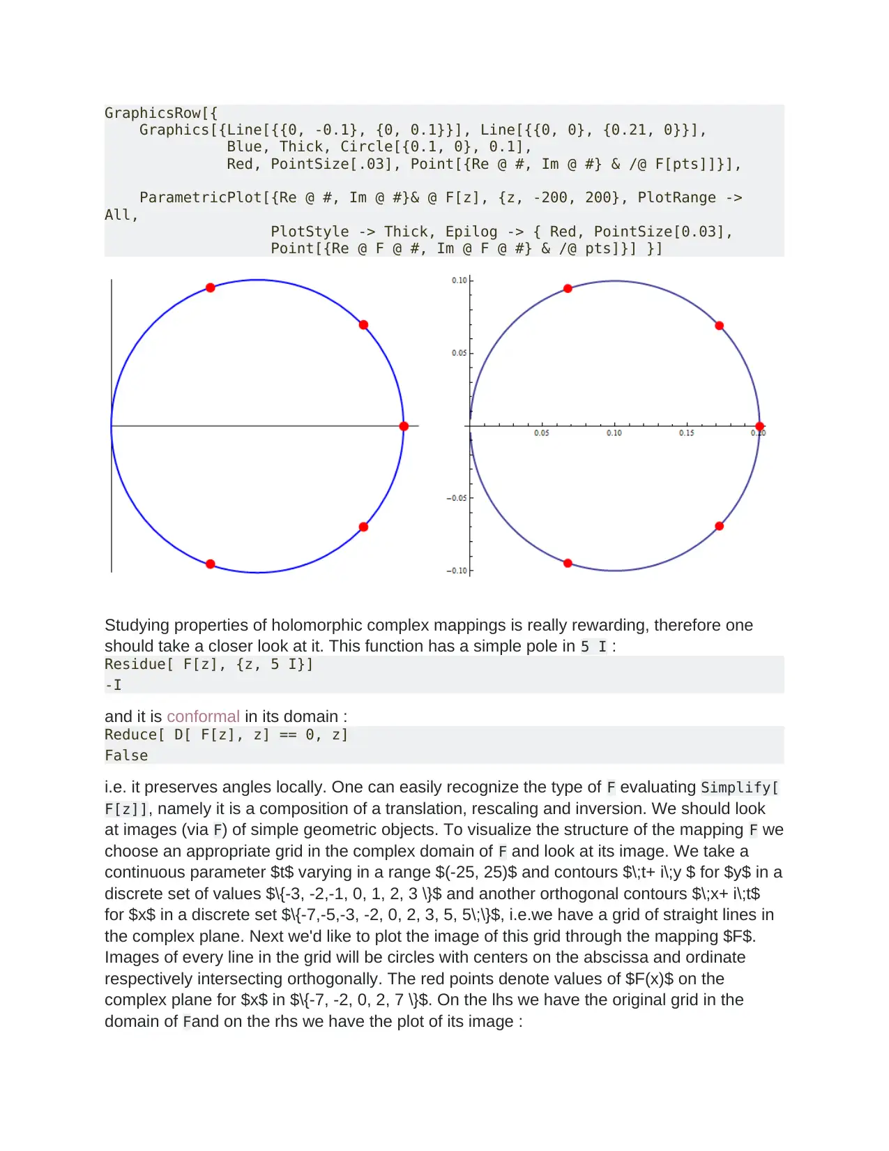
Animate[
GraphicsRow[
ParametricPlot[ ##, Evaluated -> True, PlotStyle -> Thick] & @@@ {
{ Join @@ {Table[{t, k}, {k, -3, 3}],
Table[{k, t}, {k, {-7, -5, -3, -2, 0, 2, 3, 5, 7}}]},
{t, -25, a}, PlotRange -> {{-30, 30}, {-30, 30}},
Epilog -> {Red, PointSize[0.015], Point[{#, 0} & /@ pts]} },
{ Join @@ {Table[{Re @ F[t + I k], Im @ F[t + I k]}, {k, -3, 3}],
Table[{Re @ F[k + I t], Im @ F[k + I t]},
{k, {-7, -5, -3, -2, 0, 2, 3, 5, 7}}]},
{t, -25, a}, PlotRange -> {{-.4, .6}, {-.51, .51}},
Epilog -> { Red, PointSize[0.015],
Point[{Re @ F[#], Im @ F[#]} & /@ pts]}}},
ImageSize -> 800 ], {a, -25 + 0.1, 25}]
and slightly modyfing the ranges of the last ParametricPlot : {t, -300, 300},
and PlotRange -> {{-.2, .3}, {-.25, .25}} :
ParametricPlot[
Join @@ { Table[{Re @ F[t + I k], Im @ F[t + I k]}, {k, -3, 3}],
Table[{Re @ F[k + I t], Im @ F[k + I t]},
{k, {-7, -5, -3, -2, 0, 2, 3, 5, 7}}]}, {t, -300, 300},
PlotRange -> {{-.2, .3}, {-.25, .25}}, Epilog -> {Red, PointSize[0.015],
Point[{Re @ #, Im @ #} & /@ F @ pts]},
Evaluated -> True, PlotStyle -> Thick]

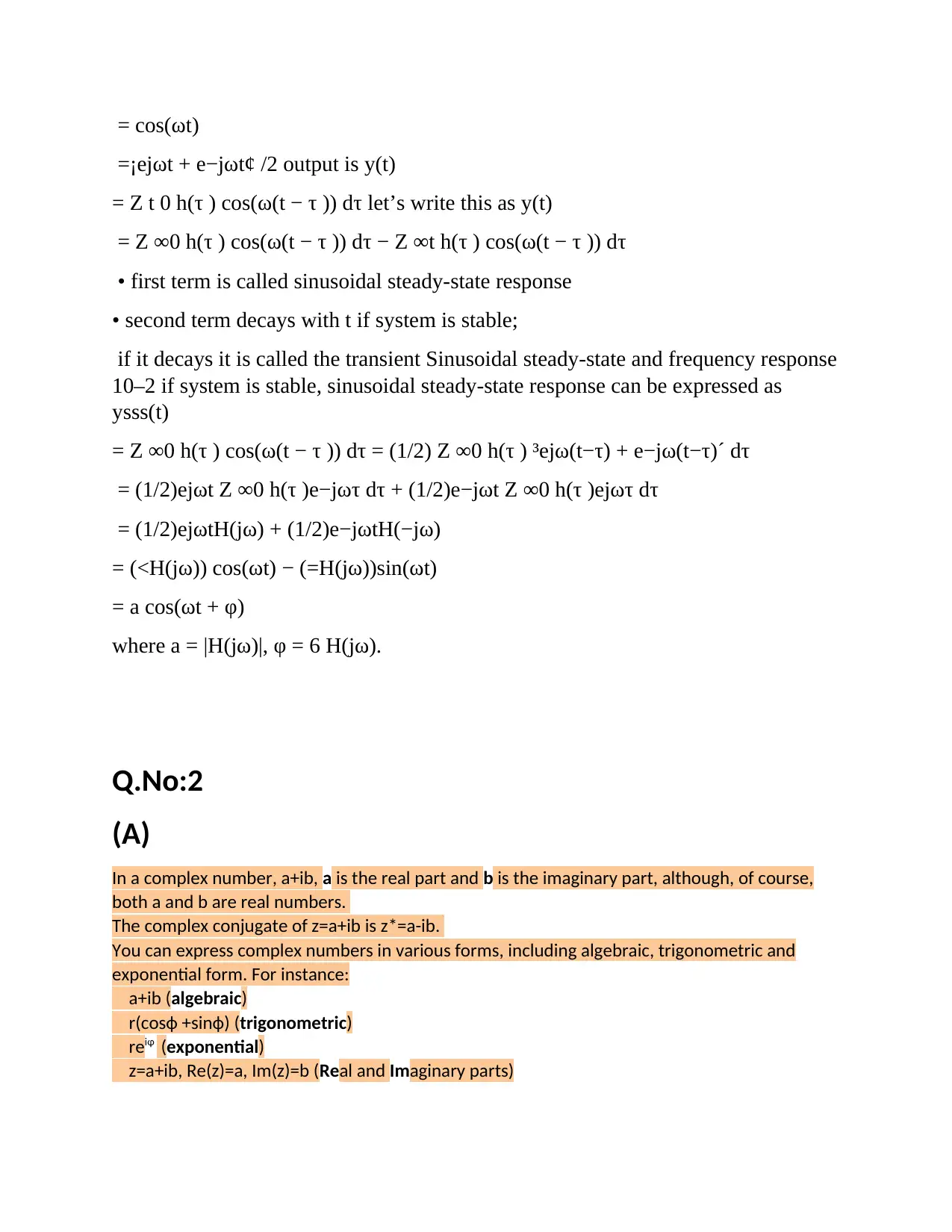
(C)
convolution system with impulse response h,
transfer function H PSfrag replacements u y H sinusoidal
input u(t)

= cos(ωt)
=¡ejωt + e−jωt¢ /2 output is y(t)
= Z t 0 h(τ ) cos(ω(t − τ )) dτ let’s write this as y(t)
= Z ∞0 h(τ ) cos(ω(t − τ )) dτ − Z ∞t h(τ ) cos(ω(t − τ )) dτ
• first term is called sinusoidal steady-state response
• second term decays with t if system is stable;
if it decays it is called the transient Sinusoidal steady-state and frequency response
10–2 if system is stable, sinusoidal steady-state response can be expressed as
ysss(t)
= Z ∞0 h(τ ) cos(ω(t − τ )) dτ = (1/2) Z ∞0 h(τ ) ³ejω(t−τ) + e−jω(t−τ)´ dτ
= (1/2)ejωt Z ∞0 h(τ )e−jωτ dτ + (1/2)e−jωt Z ∞0 h(τ )ejωτ dτ
= (1/2)ejωtH(jω) + (1/2)e−jωtH(−jω)
= (<H(jω)) cos(ωt) − (=H(jω))sin(ωt)
= a cos(ωt + φ)
where a = |H(jω)|, φ = 6 H(jω).
Q.No:2
(A)
In a complex number, a+ib, a is the real part and b is the imaginary part, although, of course,
both a and b are real numbers.
The complex conjugate of z=a+ib is z*=a-ib.
You can express complex numbers in various forms, including algebraic, trigonometric and
exponential form. For instance:
a+ib (algebraic)
r(cosф +sinф) (trigonometric)
reiφ (exponential)
z=a+ib, Re(z)=a, Im(z)=b (Real and Imaginary parts)

Complex numbers are added as follows.
Let a+ib, and c+id be a complex number, where a, b, c, and d are real numbers.
i�, or j� = – 1
(a+i�b)+(c+i�d)=(a+b) + i(b+d)
For instance:
(2+3�i)+(4+5�i)= (2+4)+(3+5)i = 6+8�i
Complex numbers often come in pairs, such as a+b�i, a–b�i and are called conjugate. If we
use z to refer to a complex number, then the conjugate is written: z*, or complex conjugate
symbol so, if:
z=a+i�b, then z*=a–i�b
Conjugate complex numbers have these properties in arithmetic:
z+z* =2a (2�Re(z) )
z-z*=2b�i (2�Im(z) )
zz*=a2 + b2 (Re(z)2 + Im(z)2 )
That is, the result has a real part only, the imaginary part vanishes.
(B)
e have `r = 5` from the question.
We must express ` θ = 135^@` in radians.
Recall:
`1^text(o)=pi/180`
So
`135^text(o)=(135pi)/180`
`=(3pi)/4`
`~~2.36` radians
So we can write
`5(cos\ 135^text(o)+j\ sin135^text(o))`
`=5e^((3pij)/4)`

` ~~ 5e^(2.36j)`
Q.No:3
(A)
Step 1:
First, the data have to be entered as matrices by listing them between brackets, leaving a space
between each entry.
X=[0.0 0.1 0.2 0.3 0.4 0.5 0.6 0.7 0.8 0.85];
ra=[0.0053 0.0052 0.005 0.0045 0.004 0.0033 0.0025 0.0018 0.00125 0.001];
4 Appendices
Step 2:
Next, the function polyfit is used to fit the data to a third-order polynomial. To learn more about the
function polyfit, type help polyfit at the command prompt.
p=polyfit(X,ra,3) (matrix of coefficients=polyfit(ind.
variable, dep. variable, order of polynomial)
p =0.0092 -0.0153 0.0013 0.0053
The coefficients are arranged in decreasing order of the independent variable of the polynomial;
therefore,
ra = 0.0092X3 – 0.0153X2 + 0.0013X = 0.0053
Please note that the typical mathematical convention for ordering coefficients is
y = a0 + a1x + a2x2 + ... + anxn whereas,
Matlab returns the solution ordered from an to a0.
Step 3:
Next, a variable f is assigned to evaluate the polynomial at the data points (i.e., f holds the ra values
calculated from the equation of the polynomial fit.)
Because X is a 1 × 10 matrix,
f will also be 1 × 10 in size.
f=polyval(p,X); f=polyval(matrix of coefficients, ind.

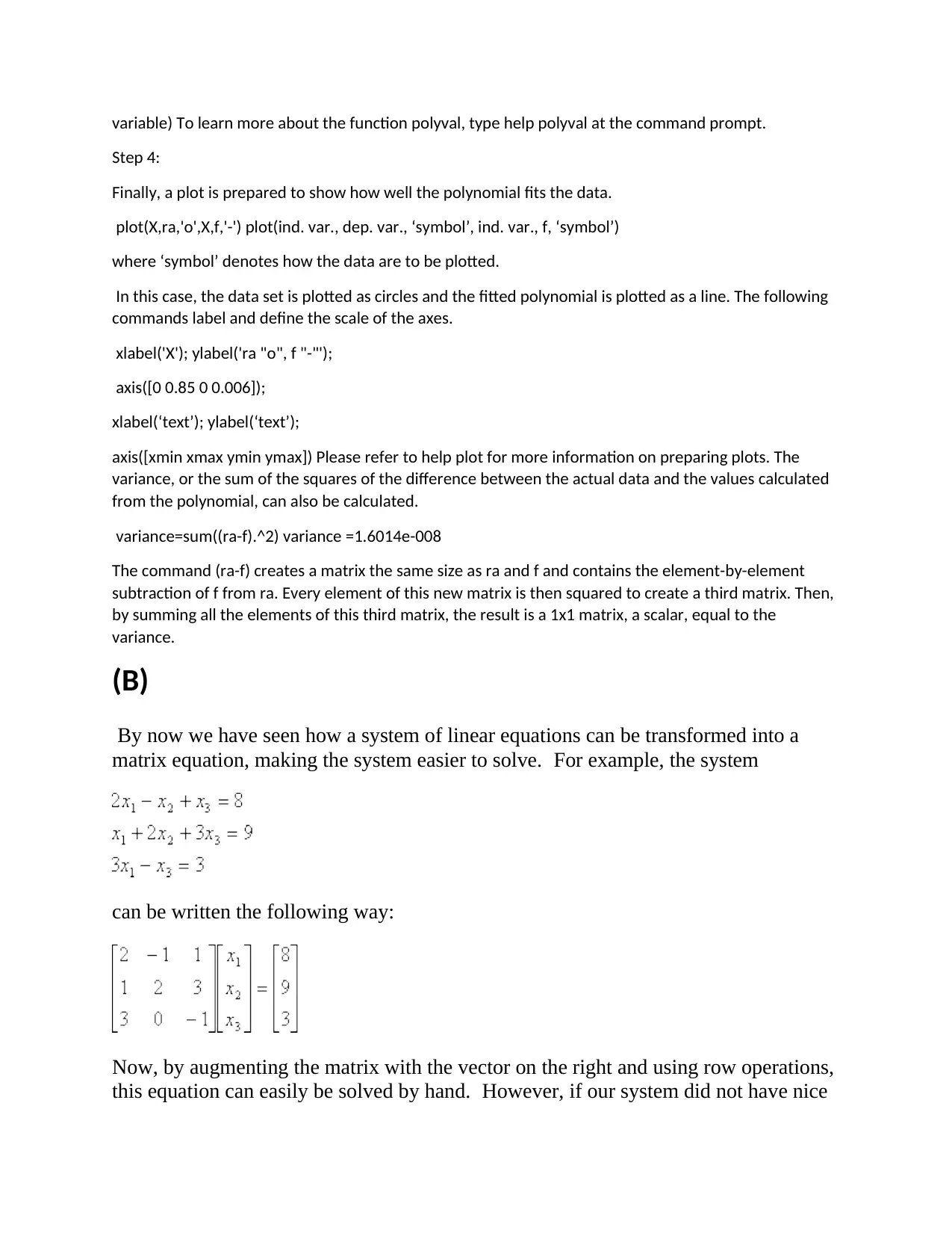
variable) To learn more about the function polyval, type help polyval at the command prompt.
Step 4:
Finally, a plot is prepared to show how well the polynomial fits the data.
plot(X,ra,'o',X,f,'-') plot(ind. var., dep. var., ‘symbol’, ind. var., f, ‘symbol’)
where ‘symbol’ denotes how the data are to be plotted.
In this case, the data set is plotted as circles and the fitted polynomial is plotted as a line. The following
commands label and define the scale of the axes.
xlabel('X'); ylabel('ra "o", f "-"');
axis([0 0.85 0 0.006]);
xlabel(‘text’); ylabel(‘text’);
axis([xmin xmax ymin ymax]) Please refer to help plot for more information on preparing plots. The
variance, or the sum of the squares of the difference between the actual data and the values calculated
from the polynomial, can also be calculated.
variance=sum((ra-f).^2) variance =1.6014e-008
The command (ra-f) creates a matrix the same size as ra and f and contains the element-by-element
subtraction of f from ra. Every element of this new matrix is then squared to create a third matrix. Then,
by summing all the elements of this third matrix, the result is a 1x1 matrix, a scalar, equal to the
variance.
(B)
By now we have seen how a system of linear equations can be transformed into a
matrix equation, making the system easier to solve. For example, the system
can be written the following way:
Now, by augmenting the matrix with the vector on the right and using row operations,
this equation can easily be solved by hand. However, if our system did not have nice

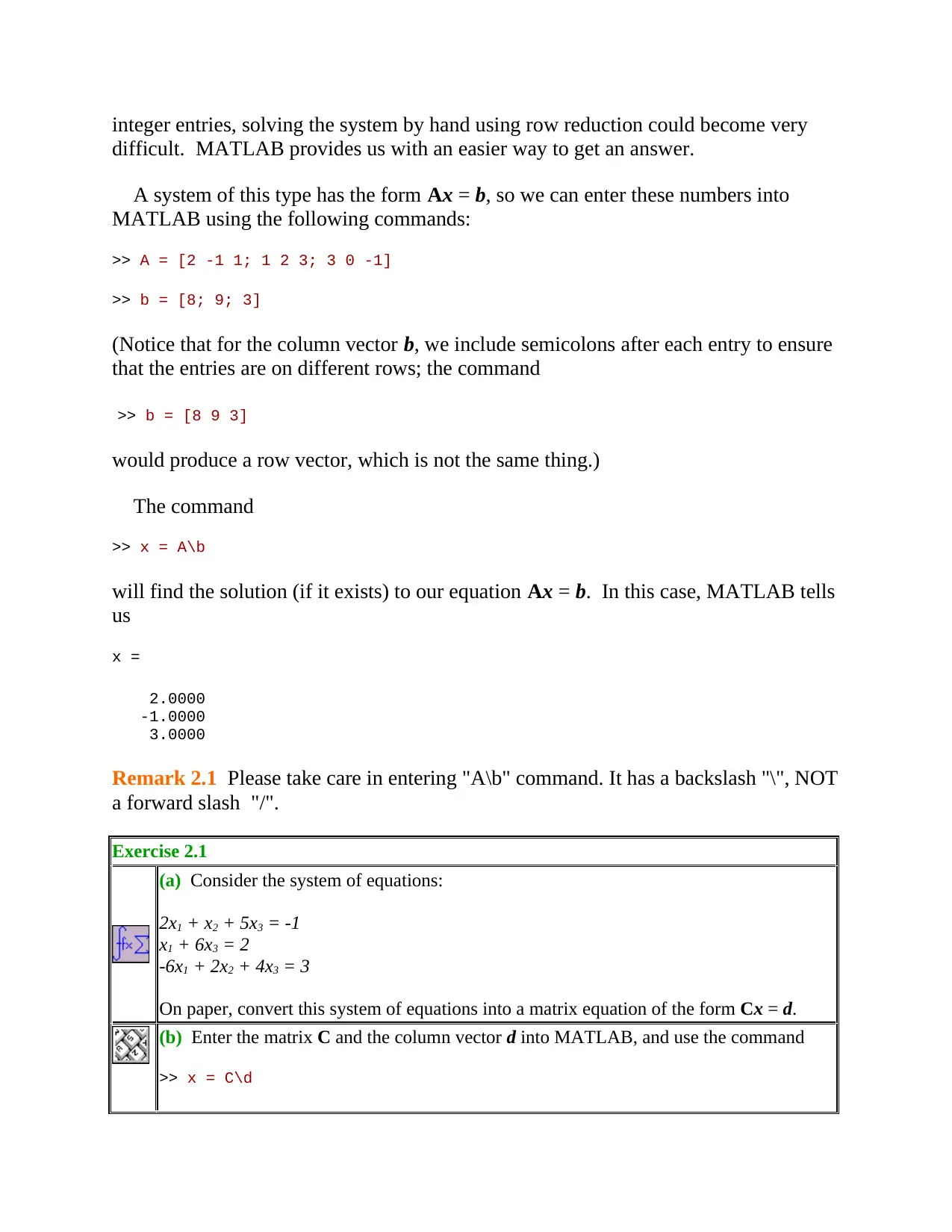
integer entries, solving the system by hand using row reduction could become very
difficult. MATLAB provides us with an easier way to get an answer.
A system of this type has the form Ax = b, so we can enter these numbers into
MATLAB using the following commands:
>> A = [2 -1 1; 1 2 3; 3 0 -1]
>> b = [8; 9; 3]
(Notice that for the column vector b, we include semicolons after each entry to ensure
that the entries are on different rows; the command
>> b = [8 9 3]
would produce a row vector, which is not the same thing.)
The command
>> x = A\b
will find the solution (if it exists) to our equation Ax = b. In this case, MATLAB tells
us
x =
2.0000
-1.0000
3.0000
Remark 2.1 Please take care in entering "A\b" command. It has a backslash "\", NOT
a forward slash "/".
Exercise 2.1
(a) Consider the system of equations:
2x1 + x2 + 5x3 = -1
x1 + 6x3 = 2
-6x1 + 2x2 + 4x3 = 3
On paper, convert this system of equations into a matrix equation of the form Cx = d.
(b) Enter the matrix C and the column vector d into MATLAB, and use the command
>> x = C\d

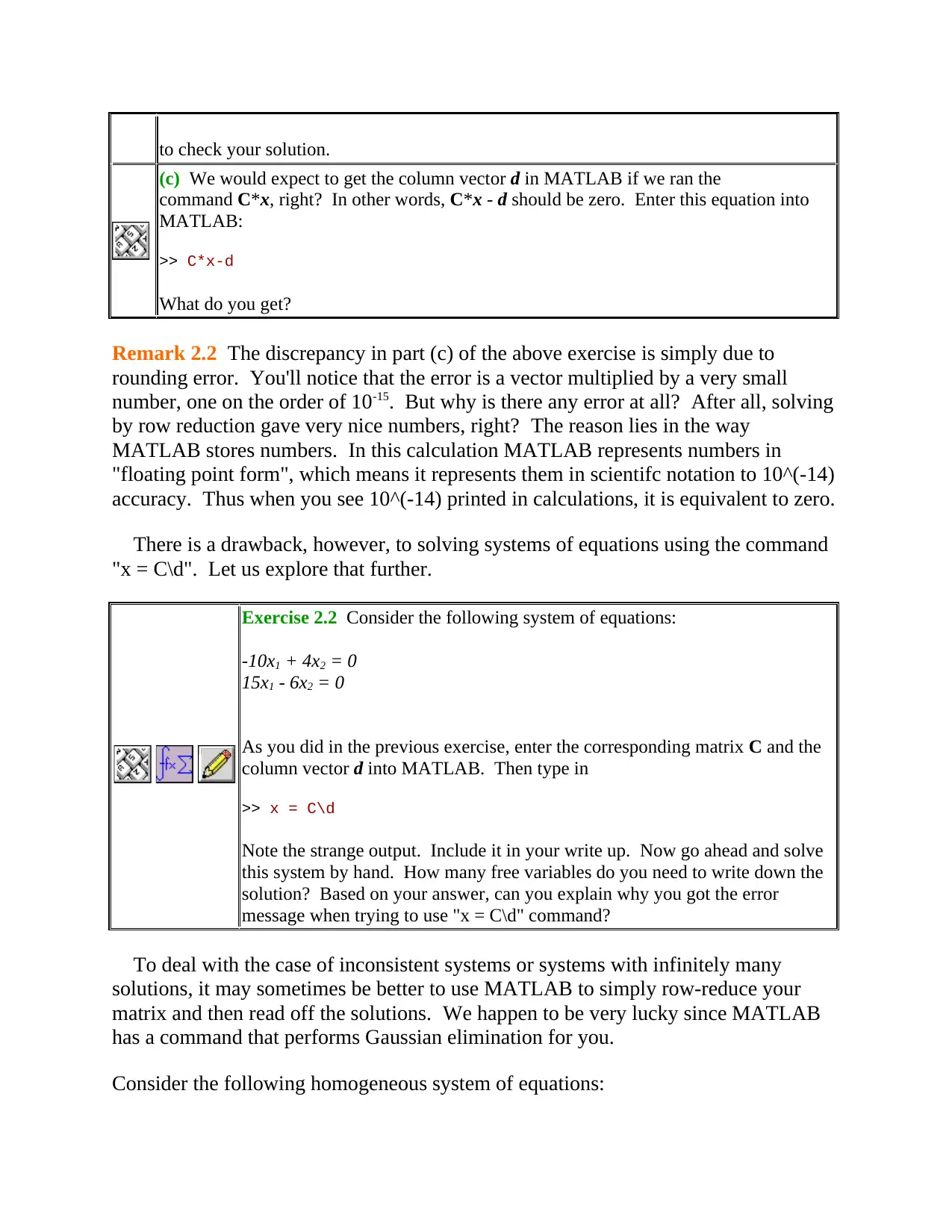
to check your solution.
(c) We would expect to get the column vector d in MATLAB if we ran the
command C*x, right? In other words, C*x - d should be zero. Enter this equation into
MATLAB:
>> C*x-d
What do you get?
Remark 2.2 The discrepancy in part (c) of the above exercise is simply due to
rounding error. You'll notice that the error is a vector multiplied by a very small
number, one on the order of 10-15. But why is there any error at all? After all, solving
by row reduction gave very nice numbers, right? The reason lies in the way
MATLAB stores numbers. In this calculation MATLAB represents numbers in
"floating point form", which means it represents them in scientifc notation to 10^(-14)
accuracy. Thus when you see 10^(-14) printed in calculations, it is equivalent to zero.
There is a drawback, however, to solving systems of equations using the command
"x = C\d". Let us explore that further.
Exercise 2.2 Consider the following system of equations:
-10x1 + 4x2 = 0
15x1 - 6x2 = 0
As you did in the previous exercise, enter the corresponding matrix C and the
column vector d into MATLAB. Then type in
>> x = C\d
Note the strange output. Include it in your write up. Now go ahead and solve
this system by hand. How many free variables do you need to write down the
solution? Based on your answer, can you explain why you got the error
message when trying to use "x = C\d" command?
To deal with the case of inconsistent systems or systems with infinitely many
solutions, it may sometimes be better to use MATLAB to simply row-reduce your
matrix and then read off the solutions. We happen to be very lucky since MATLAB
has a command that performs Gaussian elimination for you.
Consider the following homogeneous system of equations:

6x1 + 2x2 + 3x3 = 0
4x1 + x2 - 2x3 = 0
2x1 + x2 + 5x3 = 0
Enter the corresponding matrix C and the column vector d into MATLAB. Now we
want to perform row reduction on the augmented matrix [C | d]. The command that
performs row reduction in MATLAB is called "rref" (it stands for "reduced row
echelon form"). Then type in
>> rref([C d])
ans =
1.0000 0 -3.5000 0
0 1.0000 12.0000 0
0 0 0 0
Recall from class that we can then use the row reduced form to get that
x1 = 3.5x3
x2 =-12x3
x3 here is the free variable, and it can be choosen to be any value. Once chosen, the
two equations above determine the values of x1 and x2. For instance, if we choose x3 =
2, then x1 = 7 and x2 = 24. In this way we can write down all the solutions (of which
there are infinitely many) to the system above.
.
Q.No:4
(A)
The function in this example is
f(x)=3x
2
+6x−1x
2
+x−3
f =
(3*x^2 + 6*x - 1)/(x^2 + x - 3)
Plot the function f by using fplot. The fplot function automatically shows horizontal asymptotes.
ans =
3

The limit as x approaches negative infinity is also 3. This result means the line y = 3 is a horizontal
asymptote to f.
This returns the solutions to x2+x−3=0:
roots =
- 13^(1/2)/2 - 1/2
13^(1/2)/2 - 1/2
This tells you that vertical asymptotes are the lines
x=−1+G132,
and
x=−1−G132.
Find Maximum and Minimum
You can see from the graph that f has a local maximum between the points x = –2 and x = 0, and might
have a local minimum between x = –6 and x = –2. To find the x-coordinates of the maximum and
minimum, first take the derivative of f:
f1 =
(6*x + 6)/(x^2 + x - 3) - ((2*x + 1)*(3*x^2 + 6*x - 1))/(x^2 + x - 3)^2
To simplify this expression, enter
f1 = simplify(f1)
f1 =
-(3*x^2 + 16*x + 17)/(x^2 + x - 3)^2
which returns
2
3 x + 16 x + 17
- ----------------
2 2
(x + x - 3)
Next, set the derivative equal to 0 and solve for the critical points:
crit_pts = solve(f1)
crit_pts =
- 13^(1/2)/3 - 8/3
13^(1/2)/3 - 8/3
It is clear from the graph of f that it has a local minimum at
x1=−8−G133,
and a local maximum at
x2=−8+G133.
Note MATLAB® does not always return the roots to an equation in the same order.
(B)

Many different kinds of functions are used throughout mathematics and physics. Whereas some functions,
such as
f(x)=x−x36+x5120(1)
g(x)=1+x2−x28(2)
h (x) = 1 + x(3)
are polynomial functions, others, such as
u (x) = sin(x)(4)
v(x)=√1+x(5)
w(x)=11−x(6)
are not.
A function p (x) is a polynomial function of x (or in x) if it can be expressed in the form
p (x) = a0 + a1x + a2x2 + a3x3 + ... + anx n(7)
in other words, as a sum of powers of x, with each power multiplied by a coefficient (a0, a1, and so on). The
powers of xare non–negative integers.
While it is easy to see that expressions such as 1 + 2x − x2 − x3 and x5 + (x − 1)4 are polynomials in x, it is not
always so easy. For example,
(ex − e−x)2 − (ex + e−x)2 + (x sin x)2 + (x cos x)2
is actually a polynomial in x (in fact −4 + x2), but it may take a few moments thought to see why this is so.
Low-order polynomials are often given special names. Polynomials of degree zero are simply constants;
polynomials of degree one are called linear; those of degree two are called quadratic and those of degree
three are called cubic. i
An important property of any polynomial, p (x), is that for any value of x, the value of p (x) can be calculated by
simply using the arithmetic operations of addition (or subtraction) and multiplication. This is not the case with
many other functions (for example, u (x), v (x) and w (x), defined in Equations 4, 5 and 6)
u (x) = sin(x)(Eqn 4)
v(x)=1+x−−−−−√(Eqn 5)
w(x)=11−x(Eqn 6)
and it can be very useful to know polynomial approximations to such functions.
(c)
For an integration with N+1 evenly spaced points, the approximation is
b

a
f
(
x
)
dx ≈ b−a2NN

n=1
(
f
(
xn
)
+f
(
xn+1
))
=b−a2N
[
f
(
x1
)
+2f
(
x2
)
+...+2f
(
xN
)
+f
(
xN+1
)]
,
where the spacing between each point is equal to the scalar value b−aN.
If the spacing between the points is not constant, then the formula generalizes to
b

a
f
(
x
)
dx ≈ 12N

n=1
(
xn+1−xn
)[
f
(
xn
)
+f
(
xn+1
)]
,

where
(
xn+1−xn
)
is the spacing between each consecutive pair of points.
(i)
Integrals don't have to get very complicated before symbolic methods fail to work.
Consider, for example, the integral
01cos(x3+x)dx:
there are no know symbolic methods, based on indefinite integration, that can be brought to bear
on this problem.
Instead, we can sample the integrand at regular integrals and carry out an estimate
based on this. One way of doing that is to approximate the function by a sequence of
straight line segments, as in the figure. The area between each segment and the x-axis
is a trapezium, meaning that if the width of the interval is h, and the y-values at each
end of the interval areyi and yi+1, then the area of the trapezium is
2h(yi+yi+1)
The entire area between the curve and the x-axis, which is to say the integral, can be
approximated by adding together several such trapezia. If there are n trapezia, and n+1 y-values
(ordinates) running from y0 to yn, then the integral is approximately
Tn=2h(y0+2y2+2y2+ +2yn−2+2yn−1+yn)
This is called the trapezium rule.

The trapezium rule with four ordinates
For example, let us estimate
01cos(x3+x)dx
using five ordinates (four intervals). The interval width, h, is 0 25. From the table,
T4=20 25 (0 58385+2 2 16432)=0 6141
Table 1: Trapezium rule tabulation
i x_i y_1
0 0.00 1.0000
1 0.25 0.96493
2 0.50 0.81096
3 0.7 0.38843
4 1.00 -
0.41615
Totals 0.58385 2.16432
An alternative, which is often (though not always) more accurate, is to approximate the
curve with a sequence of quadratic parabolic segments instead of straight lines. Each
parabola requires three points to specify it, so each parabola spans two intervals. This
method can only be used, therefore, if the number of intervals is even (and the number
of ordinates, therefore, odd).

Figure 2: Approximating a curve (red) with a quadratic (blue): the basis of
Simpson's rule
Now, consider the quadratic passing through the points (−h y0), (0 y1) and (h y2). It's
not hard to show that this has the equation
y= 2h2y0−2y1+y2 x2+ 2hy2−y0 x+y1
If we integrate this between −h and h we get
3h(y0+4y1+y2)
This would also have been the area if we'd situated the middle of the interval somewhere other
than zero (though the calculations would have been harder). So from our quadratic
approximation we get the estimate
Sn=3h(y0+4y2+2y2+4y3+ +4yn−3+2yn−2+4yn−1+yn)
where n must be even. This is called Simpson's rule.
From the table,
Table 2: Simpson's rule tabulation
i x_i y_1
0 0.00 1.0000
1 0.25 0.9649
3
2 0.50
3 0.7 0.3884
3
4 1.00
-
0.4161
5
Total
s
0.5838
5
1.3533
5
0.8109
6
S4=30 25(0 58395+4 1 35335+2 0 81096)=0 6349

(ii)
The trapezium rule is a way of estimating the area under a curve. We know that the area
under a curve is given by integration, so the trapezium rule gives a method of estimating
integrals. This is useful when we come across integrals that we don't know how to evaluate.
The trapezium rule works by splitting the area under a curve into a number of trapeziums,
which we know the area of.
If we want to find the area under a curve between the points x0 and xn, we divide this interval
up into smaller intervals, each of which has length h (see diagram above).
Then we find that:
where y0 = f(x0) and y1 = f(x1) etc
If the original interval was split up into n smaller intervals, then h is given by: h = (xn - x0)/n
Example