Tutor Marked Exercise 3: Theory Section - Statistics and Probability

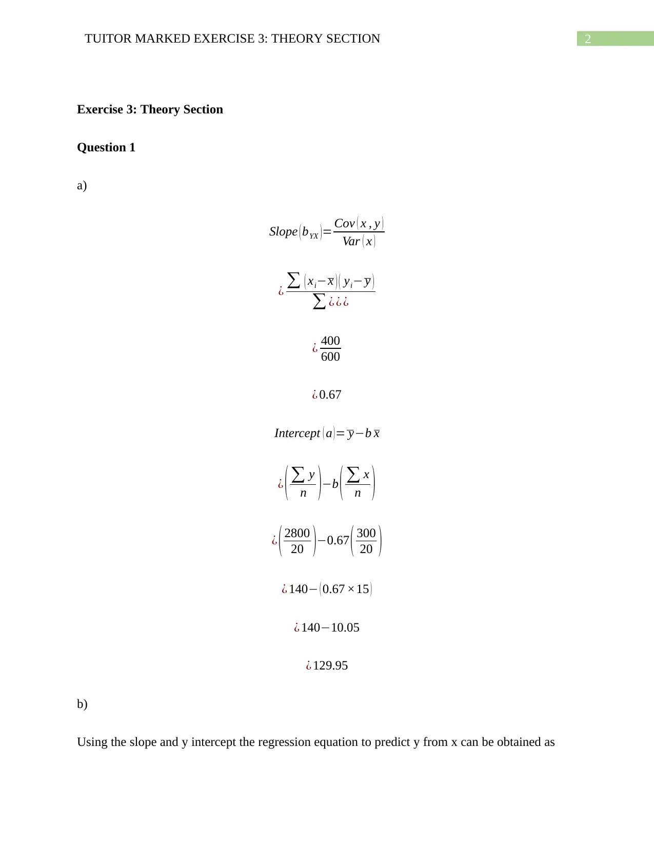
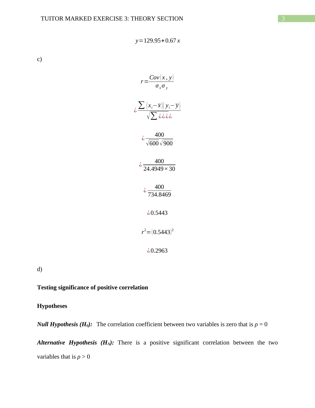
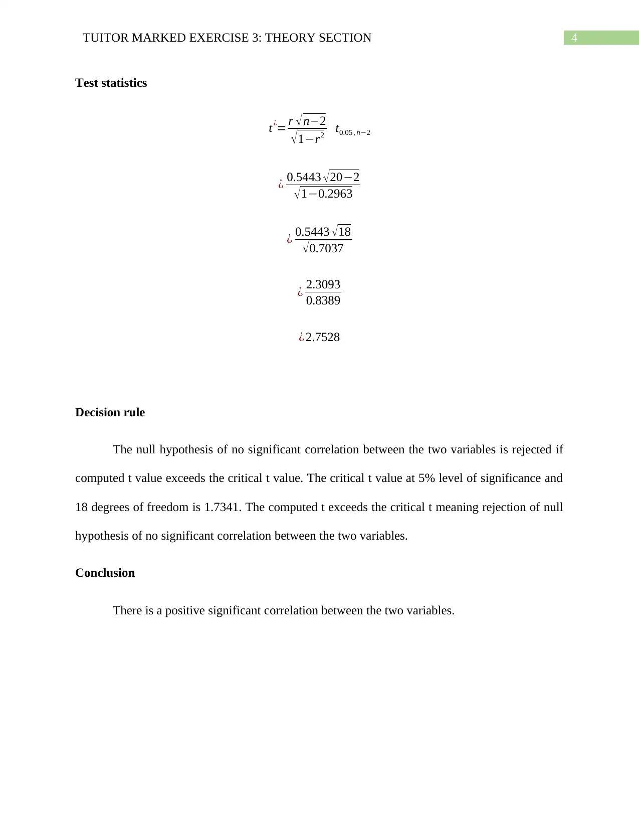
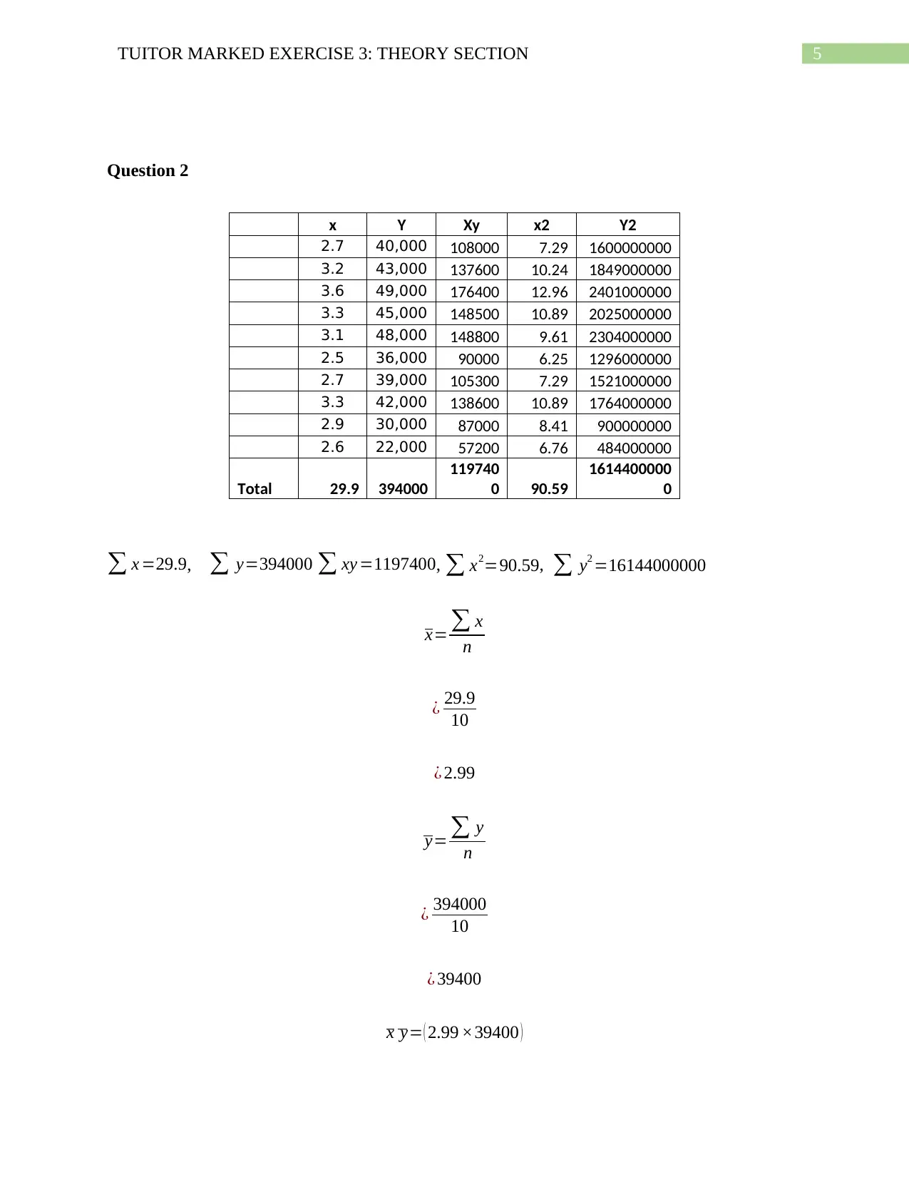
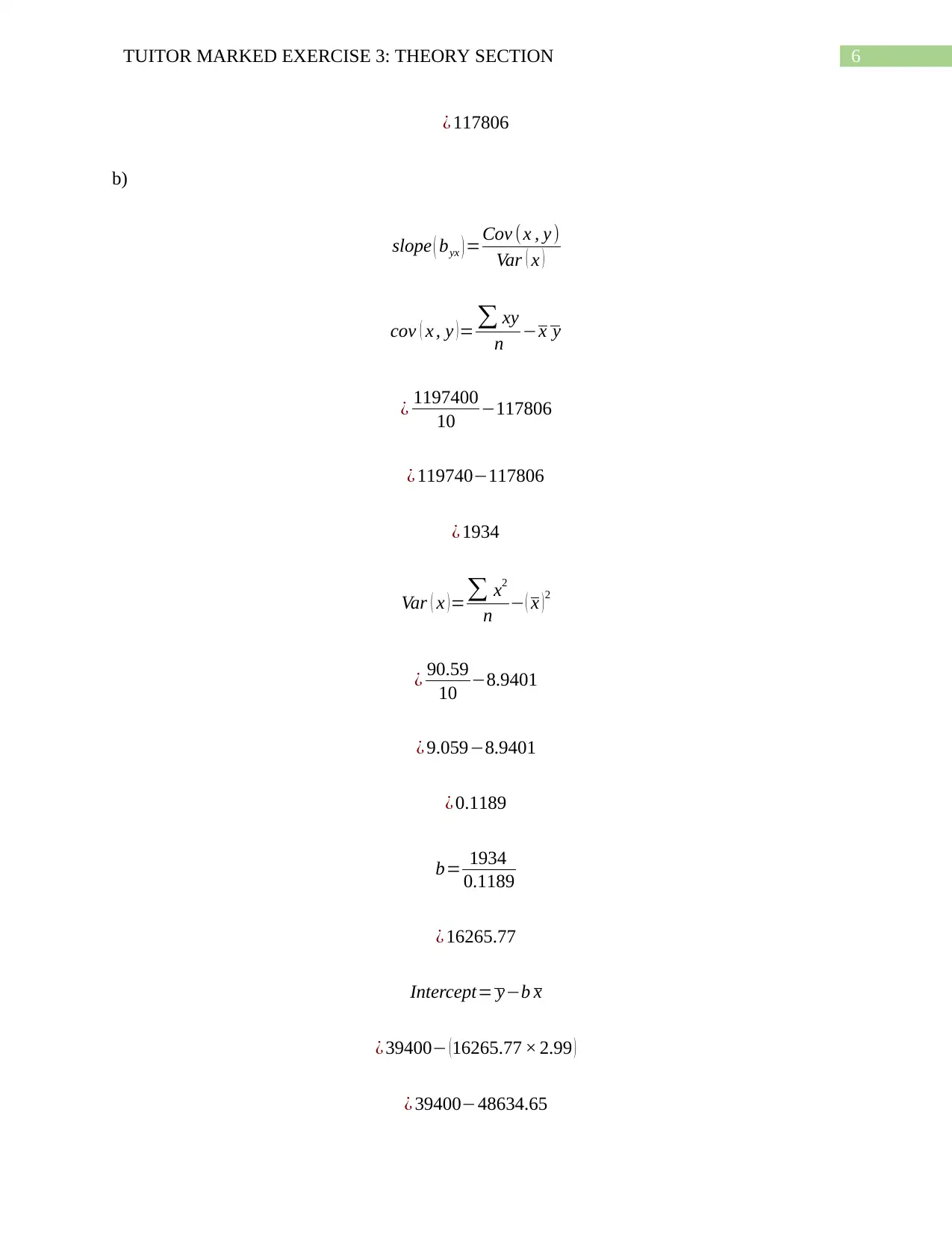
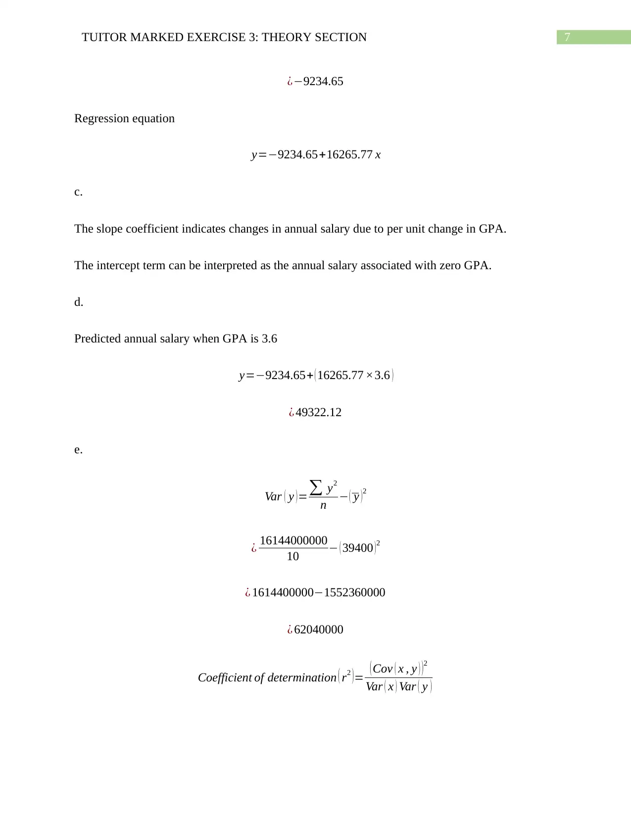
This document presents the solutions to the Theory Section of Tutor Marked Exercise 3. The assignment covers various statistical concepts, including regression analysis, hypothesis testing, and correlation. Question 1 explores regression equations, correlation significance, and hypothesis testin...Read More

Running head: TUITOR MARKED EXERCISE 3: THEORY SECTION
Tuitor Marked Exercise 3: Theory Section
Name of the Student
Name of the University
Course ID

1TUITOR MARKED EXERCISE 3: THEORY SECTION
Table of Contents
Exercise 3: Theory Section..............................................................................................................2
Question 1....................................................................................................................................2
Question 2....................................................................................................................................3
Question 3....................................................................................................................................7
Question 4....................................................................................................................................8
References......................................................................................................................................10

2TUITOR MARKED EXERCISE 3: THEORY SECTION
Exercise 3: Theory Section
Question 1
a)
Slope ( bYX )= Cov ( x , y )
Var ( x )
¿ ∑ ( xi−x )( yi− y )
∑ ¿ ¿ ¿
¿ 400
600
¿ 0.67
Intercept ( a )= y−b x
¿ ( ∑ y
n )−b ( ∑ x
n )
¿ ( 2800
20 )−0.67 ( 300
20 )
¿ 140− ( 0.67 ×15 )
¿ 140−10.05
¿ 129.95
b)
Using the slope and y intercept the regression equation to predict y from x can be obtained as

3TUITOR MARKED EXERCISE 3: THEORY SECTION
y=129.95+ 0.67 x
c)
r =Cov ( x , y )
σ x σ y
¿ ∑ ( xi−x )( yi− y )
√ ∑ ¿ ¿ ¿ ¿
¿ 400
√ 600 √ 900
¿ 400
24.4949× 30
¿ 400
734.8469
¿ 0.5443
r2= ( 0.5443 )2
¿ 0.2963
d)
Testing significance of positive correlation
Hypotheses
Null Hypothesis (H0): The correlation coefficient between two variables is zero that is ρ = 0
Alternative Hypothesis (HA): There is a positive significant correlation between the two
variables that is ρ > 0

4TUITOR MARKED EXERCISE 3: THEORY SECTION
Test statistics
t¿= r √n−2
√1−r2 t0.05 , n−2
¿ 0.5443 √ 20−2
√ 1−0.2963
¿ 0.5443 √18
√0.7037
¿ 2.3093
0.8389
¿ 2.7528
Decision rule
The null hypothesis of no significant correlation between the two variables is rejected if
computed t value exceeds the critical t value. The critical t value at 5% level of significance and
18 degrees of freedom is 1.7341. The computed t exceeds the critical t meaning rejection of null
hypothesis of no significant correlation between the two variables.
Conclusion
There is a positive significant correlation between the two variables.

5TUITOR MARKED EXERCISE 3: THEORY SECTION
Question 2
x Y Xy x2 Y2
2.7 40,000 108000 7.29 1600000000
3.2 43,000 137600 10.24 1849000000
3.6 49,000 176400 12.96 2401000000
3.3 45,000 148500 10.89 2025000000
3.1 48,000 148800 9.61 2304000000
2.5 36,000 90000 6.25 1296000000
2.7 39,000 105300 7.29 1521000000
3.3 42,000 138600 10.89 1764000000
2.9 30,000 87000 8.41 900000000
2.6 22,000 57200 6.76 484000000
Total 29.9 394000
119740
0 90.59
1614400000
0
∑ x =29.9, ∑ y=394000 ∑ xy =1197400, ∑ x2=90.59, ∑ y2 =16144000000
x= ∑ x
n
¿ 29.9
10
¿ 2.99
y= ∑ y
n
¿ 394000
10
¿ 39400
x y= ( 2.99 ×39400 )

6TUITOR MARKED EXERCISE 3: THEORY SECTION
¿ 117806
b)
slope ( byx ) =Cov (x , y )
Var ( x )
cov ( x , y ) = ∑ xy
n −x y
¿ 1197400
10 −117806
¿ 119740−117806
¿ 1934
Var ( x )=∑ x2
n − ( x )2
¿ 90.59
10 −8.9401
¿ 9.059−8.9401
¿ 0.1189
b= 1934
0.1189
¿ 16265.77
Intercept= y−b x
¿ 39400− (16265.77 × 2.99 )
¿ 39400−48634.65

7TUITOR MARKED EXERCISE 3: THEORY SECTION
¿−9234.65
Regression equation
y=−9234.65+16265.77 x
c.
The slope coefficient indicates changes in annual salary due to per unit change in GPA.
The intercept term can be interpreted as the annual salary associated with zero GPA.
d.
Predicted annual salary when GPA is 3.6
y=−9234.65+ ( 16265.77 ×3.6 )
¿ 49322.12
e.
Var ( y )=∑ y2
n − ( y )2
¿ 16144000000
10 − ( 39400 )2
¿ 1614400000−1552360000
¿ 62040000
Coefficient of determination ( r2 )= ( Cov ( x , y ) )2
Var ( x ) Var ( y )

8TUITOR MARKED EXERCISE 3: THEORY SECTION
¿ ( 1934 )2
0.1189× 62040000
¿ 0.5070 0.51
The obtained value of coefficient of determination is 0.51. This implies GPA accounts for 51
percent variation in annual salary (Chatterjee & Hadi, 2015) As a significant portion of annual
salary remain unexplained by GPA, the model is only moderately good fit.
f)
Test of slope
Hypotheses
Null Hypothesis (H0): The slope coefficient is zero that is β = 0
Alternative Hypothesis (HA): The slope coefficient is not zero that is β ≠ 0
Test statistics
t= β
S Eβ
t= 16265.77
5670.18 =2.87
The null hypothesis of zero slope coefficient is rejected if computed t value exceeds the
critical t value. The critical t value at 5% level of significance and 8 degrees of freedom is
1.8595. The computed t exceeds the critical t meaning rejection of null hypothesis of zero slope
coefficient.
g)

9TUITOR MARKED EXERCISE 3: THEORY SECTION
Test of correlation
Hypotheses
Null Hypothesis (H0): The correlation coefficient between two variables is zero that is ρ = 0
Alternative Hypothesis (HA): There is a positive significant correlation between the two
variables that is ρ > 0
Test statistics
t¿= r √n−2
√1−r2 t0.05 , n−2
¿ 0.7120 √ 10−2
√ 1−0.5070
¿ 0.7120 √8
√0.493
¿ 2.0138
0.7021
¿ 2.8683
Decision rule
The null hypothesis of no significant correlation between the two variables is rejected if
computed t value exceeds the critical t value. The critical t value at 5% level of significance and
8 degrees of freedom is 1.8595. The computed t exceeds the critical t meaning rejection of null
hypothesis of no significant correlation between the two variables.
Conclusion

10TUITOR MARKED EXERCISE 3: THEORY SECTION
There is a positive significant correlation between the two variables.
h)
The t-stat for the slope coefficient consist the standard error originated from the
independent variable and as there is only one independent variable the model also consist the
standard error of that independent variable only. This is one of the reason behind no change in
the t-stat. This also happens when the standard error of the Y and X are same.
i)
At 95% confidence interval, the range of estimated slope coefficient is 16265.769 ±
(2*5670.182)
j)
At 95% confidence interval, the range of estimated slope coefficient is 0.71208 ± (2*0.2482)
Question 3
a)

11TUITOR MARKED EXERCISE 3: THEORY SECTION
b)
F= MSregression
MSresidual
¿ 290.40000
4.36000
¿ 66.6055
The critical F value at 5% level of significance with degrees of freedom (1, 10) is 4.9646. The
computed F exceeds the critical F meaning rejection of null hypothesis that slope of the line is
zero (Schroeder, Sjoquist & Stephan, 2016). Therefore, there is sufficient evidences that slope of
the line is not zero.
c)
In order test goodness of fit of the regression model R square value needs to be
computed.

12TUITOR MARKED EXERCISE 3: THEORY SECTION
R2=1− SSRegression
SSTotal
¿ 1− 290.40000
334.00000
¿ 1−0.8695
¿ 0.1305
The R square value is very small. The explanatory variables of the model can explain only 13
percent variation in the dependent variable. The straight line therefore does not provide an
appropriate fit (Darlington & Hayes, 2016).
Question 4
In regression analysis calibration problem refers to application of known data in an
observed relationship between independent and dependent variable in order to compute other
values of the independent variable from new observation for the explained variable. This is
termed as inverse regression.
The inverse regression analysis is a useful tool for reducing dimension in multivariate
statistics. Regression analysis is considered as a popular way of evaluating the relation between
explanatory variable and response variable (Pan & Dias, 2017). The explanatory variable is a p
dimensional vector. Several approaches generally come under the term regression. In case of
high dimensional explanatory variable, the number of dimension needs to be reduced to make the
regression operation computable. It actually aims to show the most important dimension of the
data set. Here comes the importance of inverse regression. It normally uses a regression curve

13TUITOR MARKED EXERCISE 3: THEORY SECTION
denotes as E (x|y) for performing weighted principle component analysis. Using this one can
identify an effective tool for reducing dimension.

14TUITOR MARKED EXERCISE 3: THEORY SECTION
References
Chatterjee, S., & Hadi, A. S. (2015). Regression analysis by example. John Wiley & Sons.
Darlington, R. B., & Hayes, A. F. (2016). Regression analysis and linear models: Concepts,
applications, and implementation. Guilford Publications.
Pan, Q., & Dias, D. (2017). Sliced inverse regression-based sparse polynomial chaos expansions
for reliability analysis in high dimensions. Reliability Engineering & System Safety, 167,
484-493.
Schroeder, L. D., Sjoquist, D. L., & Stephan, P. E. (2016). Understanding regression analysis:
An introductory guide (Vol. 57). Sage Publications