Study of Unemployment in Australia and New Zealand

This study analyzes the unemployment rate in Australia and New Zealand, including factors affecting it. It also studies the relationship between school enrollment, tertiary (% gross) and unemployment rate. The data is collected from the World Bank. Useful for socialists, demographers, researchers, and academicians.

Study of Unemployment in Australia and New Zealand
Author Name: Student Name

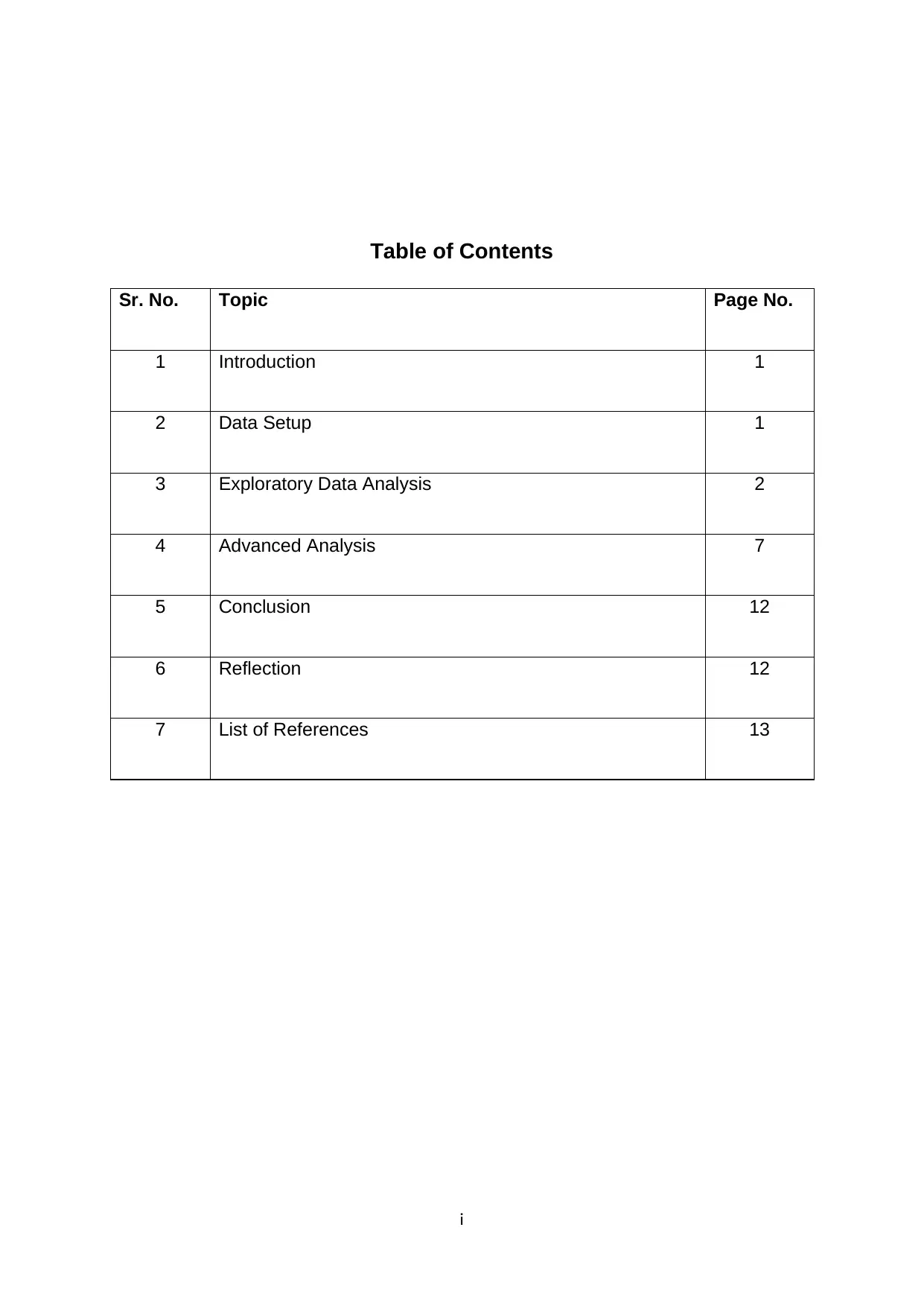
Table of Contents
Sr. No. Topic Page No.
1 Introduction 1
2 Data Setup 1
3 Exploratory Data Analysis 2
4 Advanced Analysis 7
5 Conclusion 12
6 Reflection 12
7 List of References 13
i

Study of Unemployment in Australia and New Zealand
1. Introduction
Unemployment is the situation in which people actively seeking for
employment but not getting it. Unemployment rate can be calculated by number of
people seeking for employment divided by labor force.
The unemployment rate has its own impact on countries growth. There are
various factors affecting unemployment. The unemployment rate is more in
developing and developing countries than developed countries. In this study, we
studied the unemployment rate in Australia and New Zealand. We also studied the
relationship between School enrollment, tertiary (% gross) and unemployment rate.
We group the countries using k-means cluster analysis by unemployment rate.
This study may be useful for Socialist, demographer, researchers and
academicians. Data is collected from World Bank (http://databank.worldbank.org).
2. Data Setup
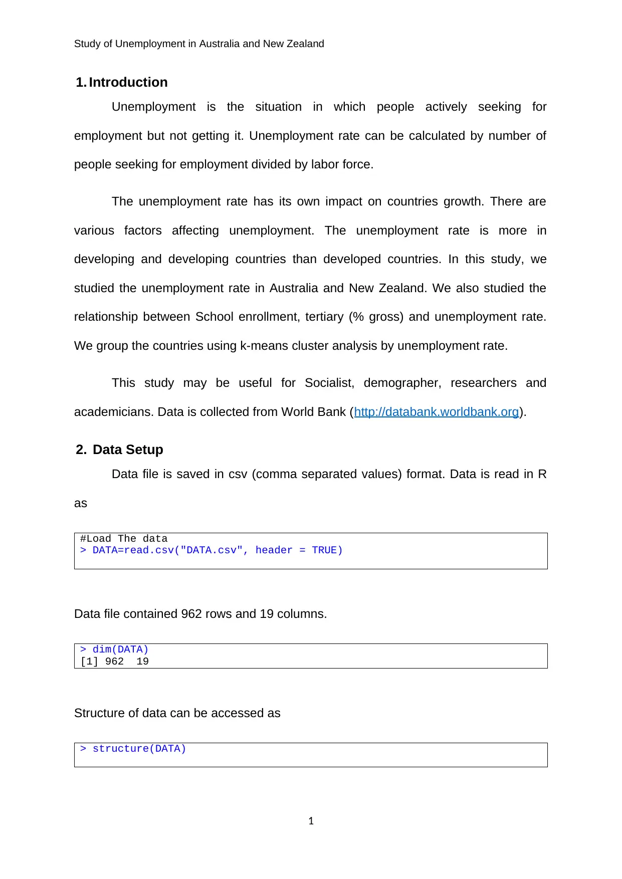
Data file is saved in csv (comma separated values) format. Data is read in R
as
#Load The data
> DATA=read.csv("DATA.csv", header = TRUE)
Data file contained 962 rows and 19 columns.
> dim(DATA)
[1] 962 19
Structure of data can be accessed as
> structure(DATA)
1

Study of Unemployment in Australia and New Zealand
3. Exploratory Data Analysis
We used dplyr library for required data extraction. Firstly library is loaded as
# Library for the required data extraction
> library(dplyr)
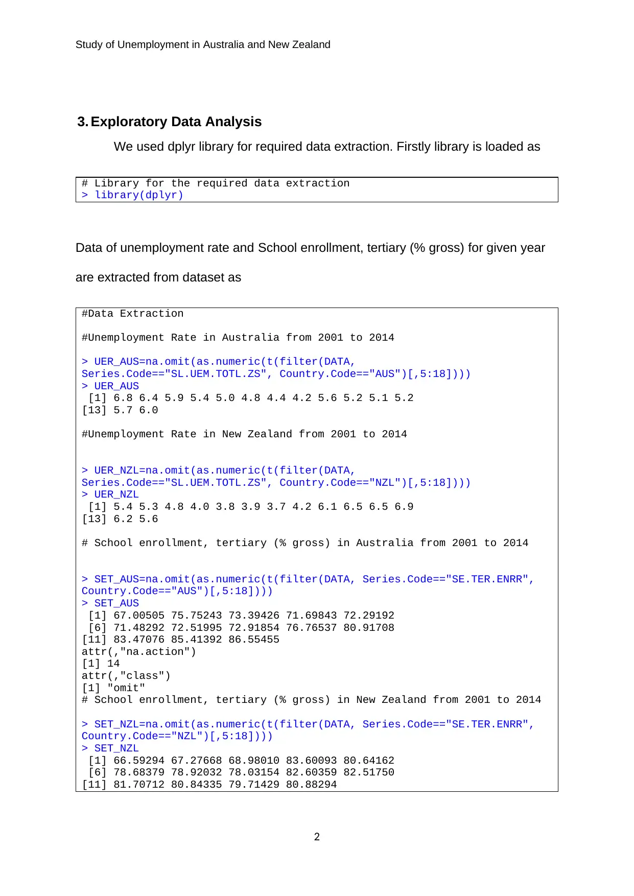
Data of unemployment rate and School enrollment, tertiary (% gross) for given year
are extracted from dataset as
#Data Extraction
#Unemployment Rate in Australia from 2001 to 2014
> UER_AUS=na.omit(as.numeric(t(filter(DATA,
Series.Code=="SL.UEM.TOTL.ZS", Country.Code=="AUS")[,5:18])))
> UER_AUS
[1] 6.8 6.4 5.9 5.4 5.0 4.8 4.4 4.2 5.6 5.2 5.1 5.2
[13] 5.7 6.0
#Unemployment Rate in New Zealand from 2001 to 2014
> UER_NZL=na.omit(as.numeric(t(filter(DATA,
Series.Code=="SL.UEM.TOTL.ZS", Country.Code=="NZL")[,5:18])))
> UER_NZL
[1] 5.4 5.3 4.8 4.0 3.8 3.9 3.7 4.2 6.1 6.5 6.5 6.9
[13] 6.2 5.6
# School enrollment, tertiary (% gross) in Australia from 2001 to 2014
> SET_AUS=na.omit(as.numeric(t(filter(DATA, Series.Code=="SE.TER.ENRR",
Country.Code=="AUS")[,5:18])))
> SET_AUS
[1] 67.00505 75.75243 73.39426 71.69843 72.29192
[6] 71.48292 72.51995 72.91854 76.76537 80.91708
[11] 83.47076 85.41392 86.55455
attr(,"na.action")
[1] 14
attr(,"class")
[1] "omit"
# School enrollment, tertiary (% gross) in New Zealand from 2001 to 2014
> SET_NZL=na.omit(as.numeric(t(filter(DATA, Series.Code=="SE.TER.ENRR",
Country.Code=="NZL")[,5:18])))
> SET_NZL
[1] 66.59294 67.27668 68.98010 83.60093 80.64162
[6] 78.68379 78.92032 78.03154 82.60359 82.51750
[11] 81.70712 80.84335 79.71429 80.88294
2

Study of Unemployment in Australia and New Zealand
We referred Hopkins, Glass and Hopkins (1987), Larsen and Marx (2017),
Hoel (1954), Berenson(2012), Bickel and Doksum (2015), Casella and Burger
(2002), DeGroot and Schervish (2012), Devore and Berk (2007), Groebner et al.
(2008) and Ross (2014), Hogg and Craig (1995) and Serfling (2009).
One Variable Analysis:
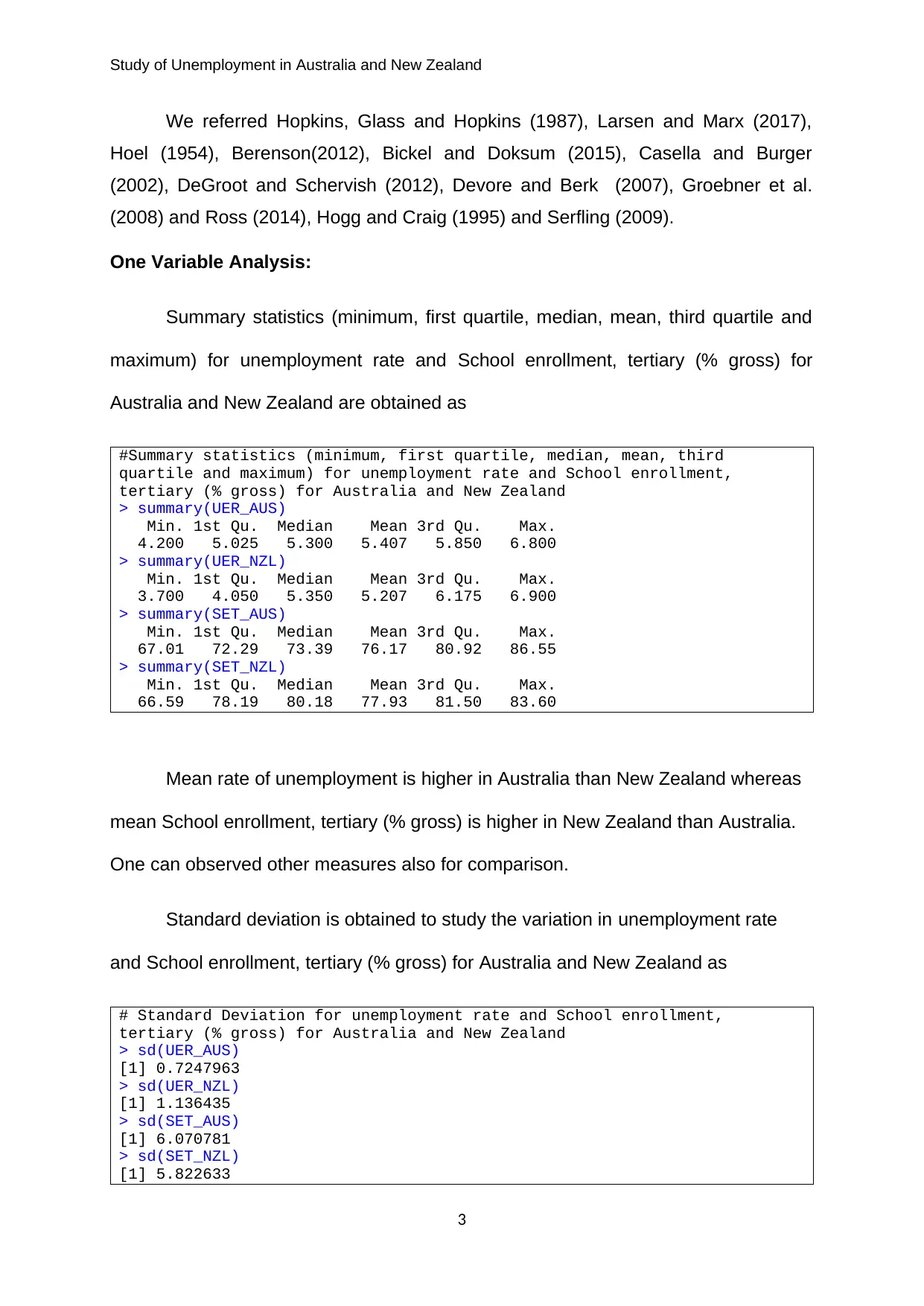
Summary statistics (minimum, first quartile, median, mean, third quartile and
maximum) for unemployment rate and School enrollment, tertiary (% gross) for
Australia and New Zealand are obtained as
#Summary statistics (minimum, first quartile, median, mean, third
quartile and maximum) for unemployment rate and School enrollment,
tertiary (% gross) for Australia and New Zealand
> summary(UER_AUS)
Min. 1st Qu. Median Mean 3rd Qu. Max.
4.200 5.025 5.300 5.407 5.850 6.800
> summary(UER_NZL)
Min. 1st Qu. Median Mean 3rd Qu. Max.
3.700 4.050 5.350 5.207 6.175 6.900
> summary(SET_AUS)
Min. 1st Qu. Median Mean 3rd Qu. Max.
67.01 72.29 73.39 76.17 80.92 86.55
> summary(SET_NZL)
Min. 1st Qu. Median Mean 3rd Qu. Max.
66.59 78.19 80.18 77.93 81.50 83.60
Mean rate of unemployment is higher in Australia than New Zealand whereas
mean School enrollment, tertiary (% gross) is higher in New Zealand than Australia.
One can observed other measures also for comparison.
Standard deviation is obtained to study the variation in unemployment rate
and School enrollment, tertiary (% gross) for Australia and New Zealand as
# Standard Deviation for unemployment rate and School enrollment,
tertiary (% gross) for Australia and New Zealand
> sd(UER_AUS)
[1] 0.7247963
> sd(UER_NZL)
[1] 1.136435
> sd(SET_AUS)
[1] 6.070781
> sd(SET_NZL)
[1] 5.822633
3

Study of Unemployment in Australia and New Zealand
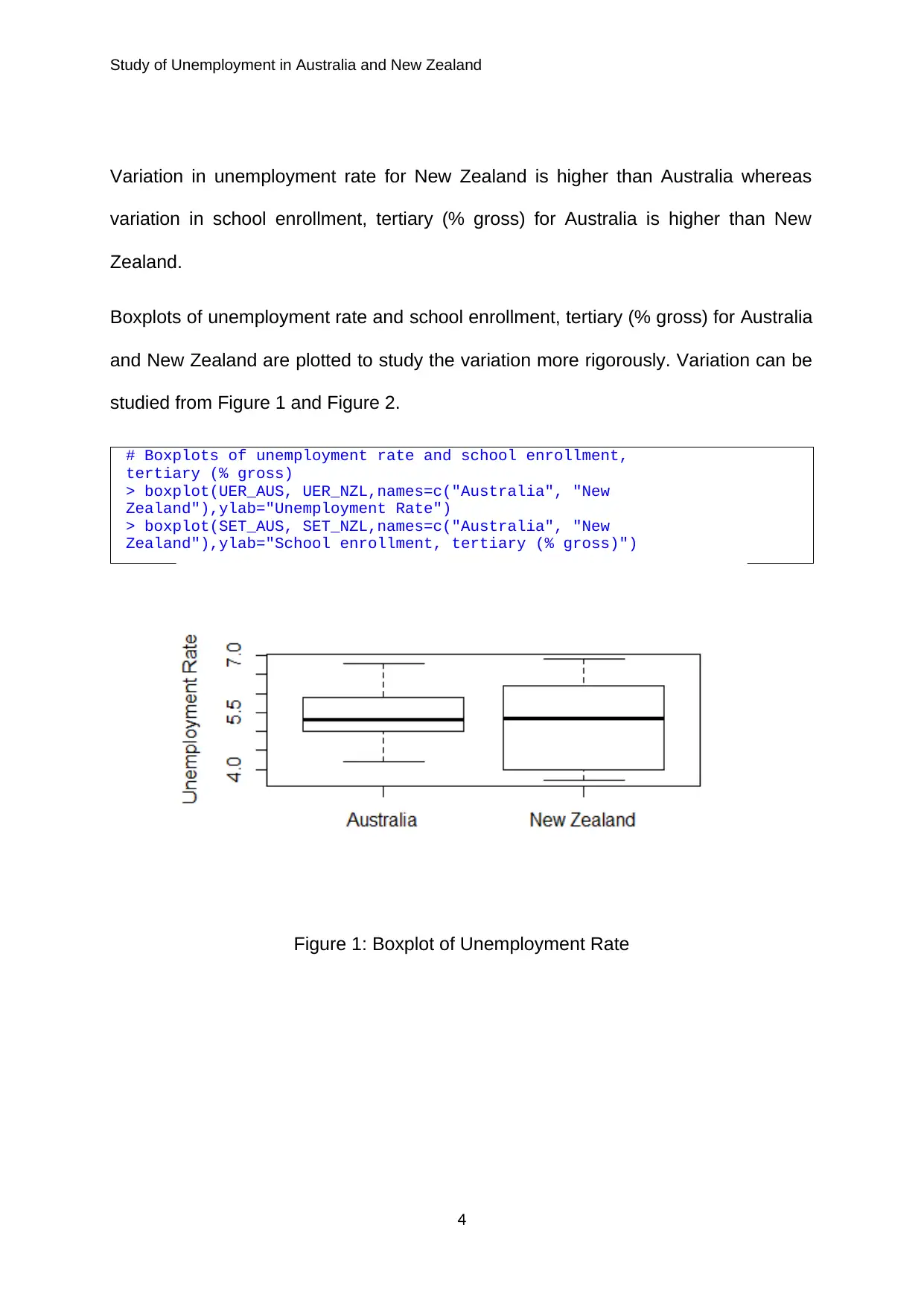
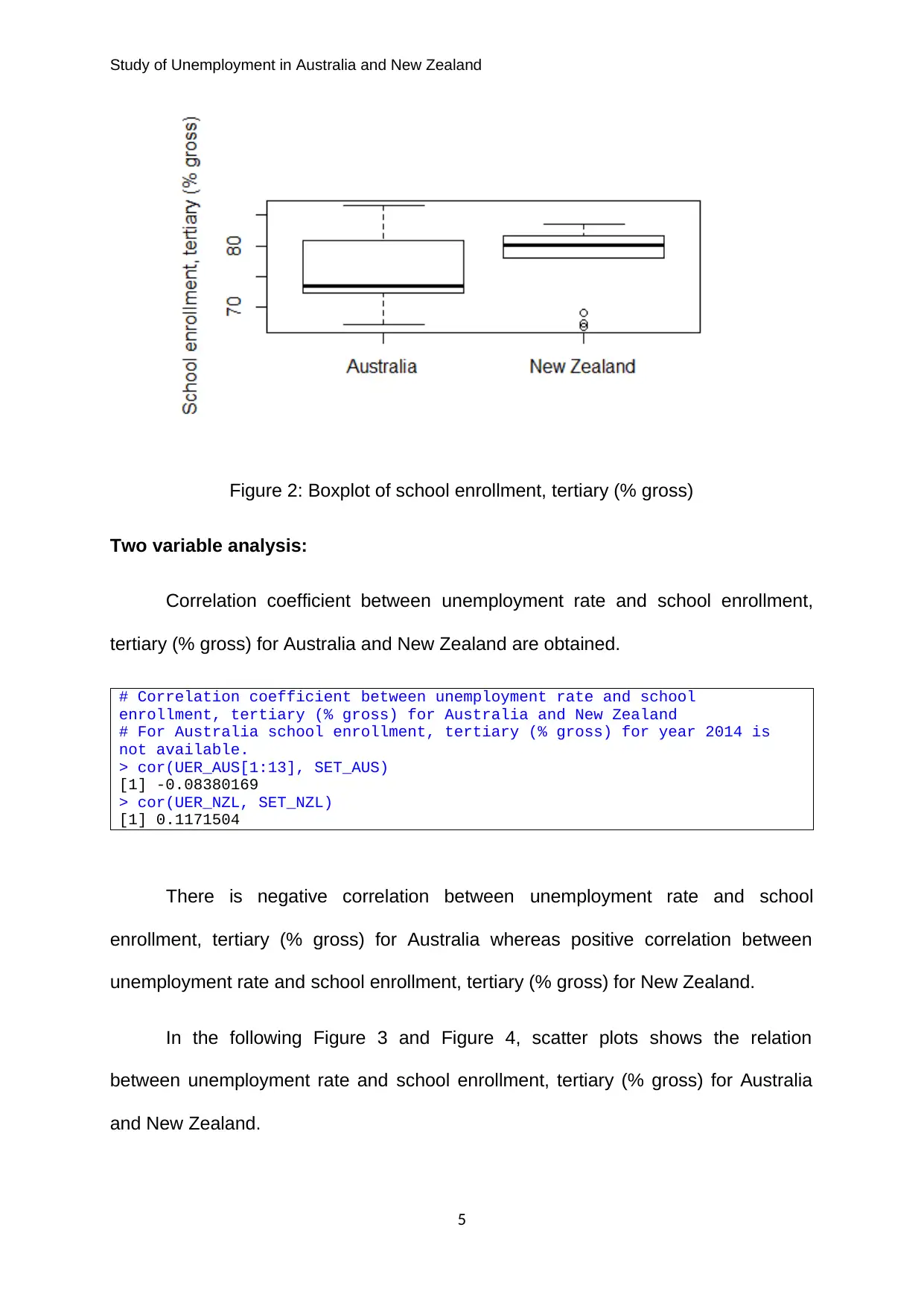
Variation in unemployment rate for New Zealand is higher than Australia whereas
variation in school enrollment, tertiary (% gross) for Australia is higher than New
Zealand.
Boxplots of unemployment rate and school enrollment, tertiary (% gross) for Australia
and New Zealand are plotted to study the variation more rigorously. Variation can be
studied from Figure 1 and Figure 2.
# Boxplots of unemployment rate and school enrollment,
tertiary (% gross)
> boxplot(UER_AUS, UER_NZL,names=c("Australia", "New
Zealand"),ylab="Unemployment Rate")
> boxplot(SET_AUS, SET_NZL,names=c("Australia", "New
Zealand"),ylab="School enrollment, tertiary (% gross)")
Figure 1: Boxplot of Unemployment Rate
4

Study of Unemployment in Australia and New Zealand
Figure 2: Boxplot of school enrollment, tertiary (% gross)
Two variable analysis:
Correlation coefficient between unemployment rate and school enrollment,
tertiary (% gross) for Australia and New Zealand are obtained.
# Correlation coefficient between unemployment rate and school
enrollment, tertiary (% gross) for Australia and New Zealand
# For Australia school enrollment, tertiary (% gross) for year 2014 is
not available.
> cor(UER_AUS[1:13], SET_AUS)
[1] -0.08380169
> cor(UER_NZL, SET_NZL)
[1] 0.1171504
There is negative correlation between unemployment rate and school
enrollment, tertiary (% gross) for Australia whereas positive correlation between
unemployment rate and school enrollment, tertiary (% gross) for New Zealand.
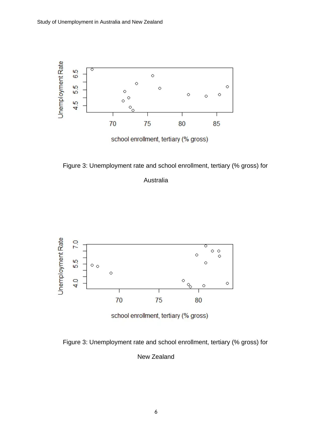
In the following Figure 3 and Figure 4, scatter plots shows the relation
between unemployment rate and school enrollment, tertiary (% gross) for Australia
and New Zealand.
5

Study of Unemployment in Australia and New Zealand
Figure 3: Unemployment rate and school enrollment, tertiary (% gross) for
Australia
Figure 3: Unemployment rate and school enrollment, tertiary (% gross) for
New Zealand
6

Study of Unemployment in Australia and New Zealand
From Figure 3 and 4, we reported that
 As school enrollment, tertiary (% gross) increases unemployment rate also
increases for New Zealand.
 As school enrollment, tertiary (% gross) increases unemployment rate
decreases for Australia.
4. Advanced Analysis
k-means clustering and linear regression are carried in this section. We
referred
Romesburg (2004) and Kaufman and Rousseeuw (2009)
4.1 Clustering
Clustering is technique of grouping. In clustering we group (cluster) the set of
objects which is similar in some characteristic than other group (cluster). In k-means
clustering is the gropuing technique where we make the k groups.
k-means clustering according to unemployment rate for year 2014 for East Asia and
Pacific countries:
First step is data extraction. Data of unemployment rate for all East Asia and Pacific
countries for year 2014 is extracted as
# Data Extration
> fd1=filter(DATA, Series.Code=="SL.UEM.TOTL.ZS")
> Country_Name=fd1$Country.Name
> UER_2014=fd1$X2014..YR2014.
> fd2=data.frame(Country_Name,UER_2014)
> fd3=subset(fd2,fd2$UER_2014!=UER_2014[1])
> UER_2014=fd3$UER_2014
> UER_2014
[1] 6.0 3.8 0.4 4.7 7.9 3.2 6.2 3.7 4.1 3.5 1.4 1.5
7

Study of Unemployment in Australia and New Zealand
[13] 2.0 4.8 3.3 5.6 2.5 7.1 3.0 3.9 0.9 4.7 2.3
> Country=fd3$Country_Name
> Country
[1] Australia
[2] Brunei Darussalam
[3] Cambodia
[4] China
[5] Fiji
[6] Hong Kong SAR, China
[7] Indonesia
[8] Japan
[9] Korea, Dem. People’s Rep.
[10] Korea, Rep.
[11] Lao PDR
[12] Macao SAR, China
[13] Malaysia
[14] Mongolia
[15] Myanmar
[16] New Zealand
[17] Papua New Guinea
[18] Philippines
[19] Singapore
[20] Solomon Islands
[21] Thailand
[22] Timor-Leste
[23] Vietnam
38 Levels: American Samoa ... Vietnam
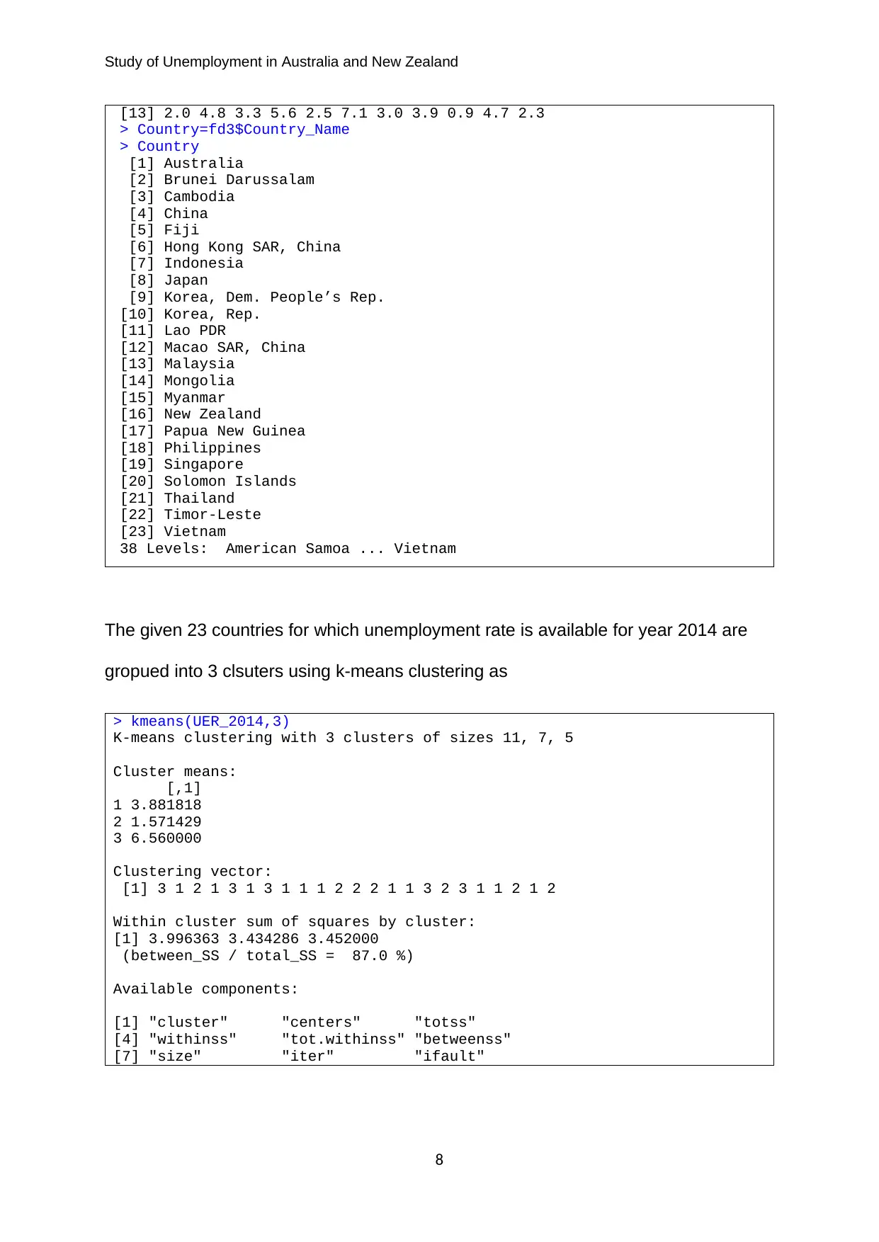
The given 23 countries for which unemployment rate is available for year 2014 are
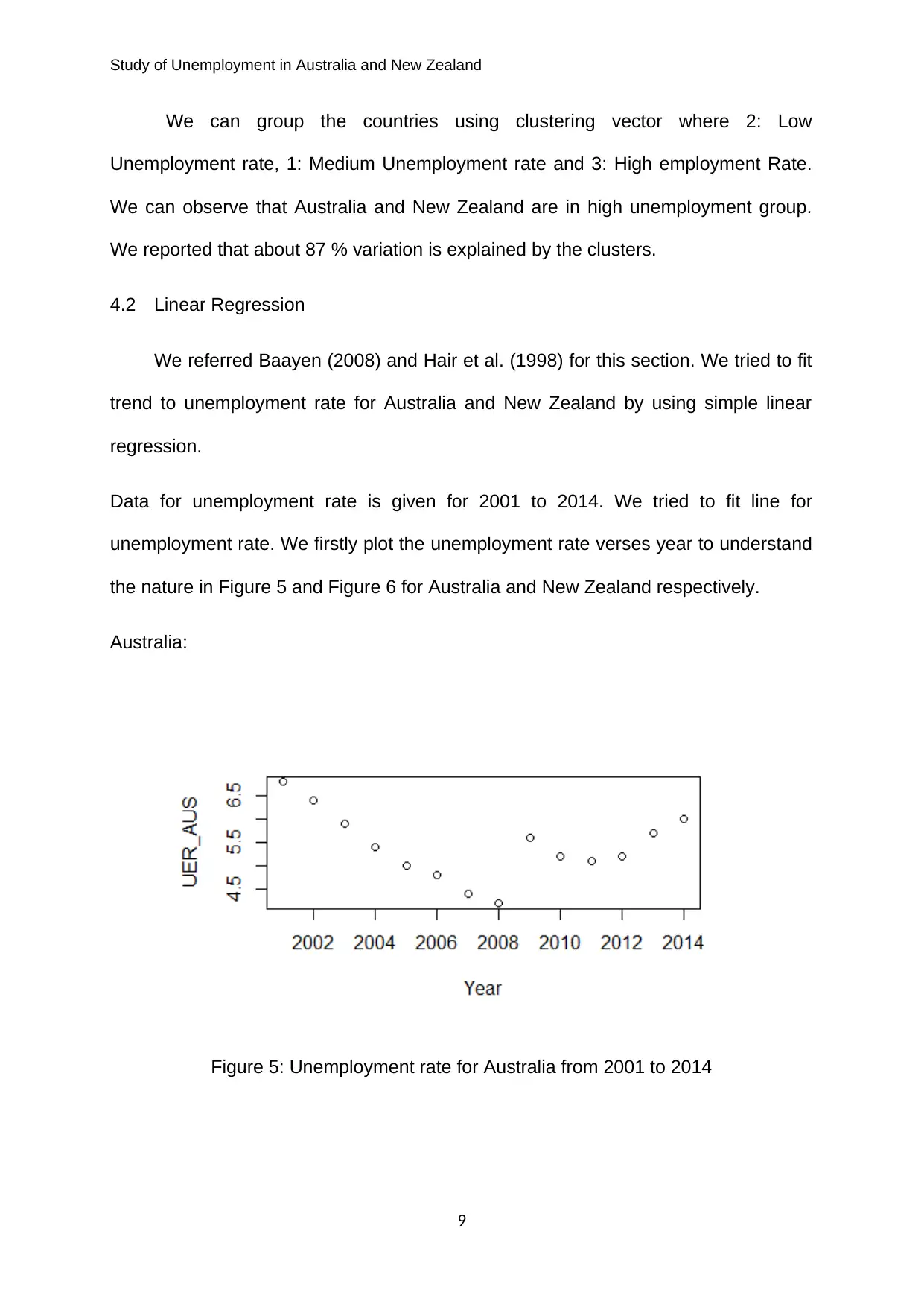
gropued into 3 clsuters using k-means clustering as
> kmeans(UER_2014,3)
K-means clustering with 3 clusters of sizes 11, 7, 5
Cluster means:
[,1]
1 3.881818
2 1.571429
3 6.560000
Clustering vector:
[1] 3 1 2 1 3 1 3 1 1 1 2 2 2 1 1 3 2 3 1 1 2 1 2
Within cluster sum of squares by cluster:
[1] 3.996363 3.434286 3.452000
(between_SS / total_SS = 87.0 %)
Available components:
[1] "cluster" "centers" "totss"
[4] "withinss" "tot.withinss" "betweenss"
[7] "size" "iter" "ifault"
8

Study of Unemployment in Australia and New Zealand
We can group the countries using clustering vector where 2: Low
Unemployment rate, 1: Medium Unemployment rate and 3: High employment Rate.
We can observe that Australia and New Zealand are in high unemployment group.
We reported that about 87 % variation is explained by the clusters.
4.2 Linear Regression
We referred Baayen (2008) and Hair et al. (1998) for this section. We tried to fit
trend to unemployment rate for Australia and New Zealand by using simple linear
regression.
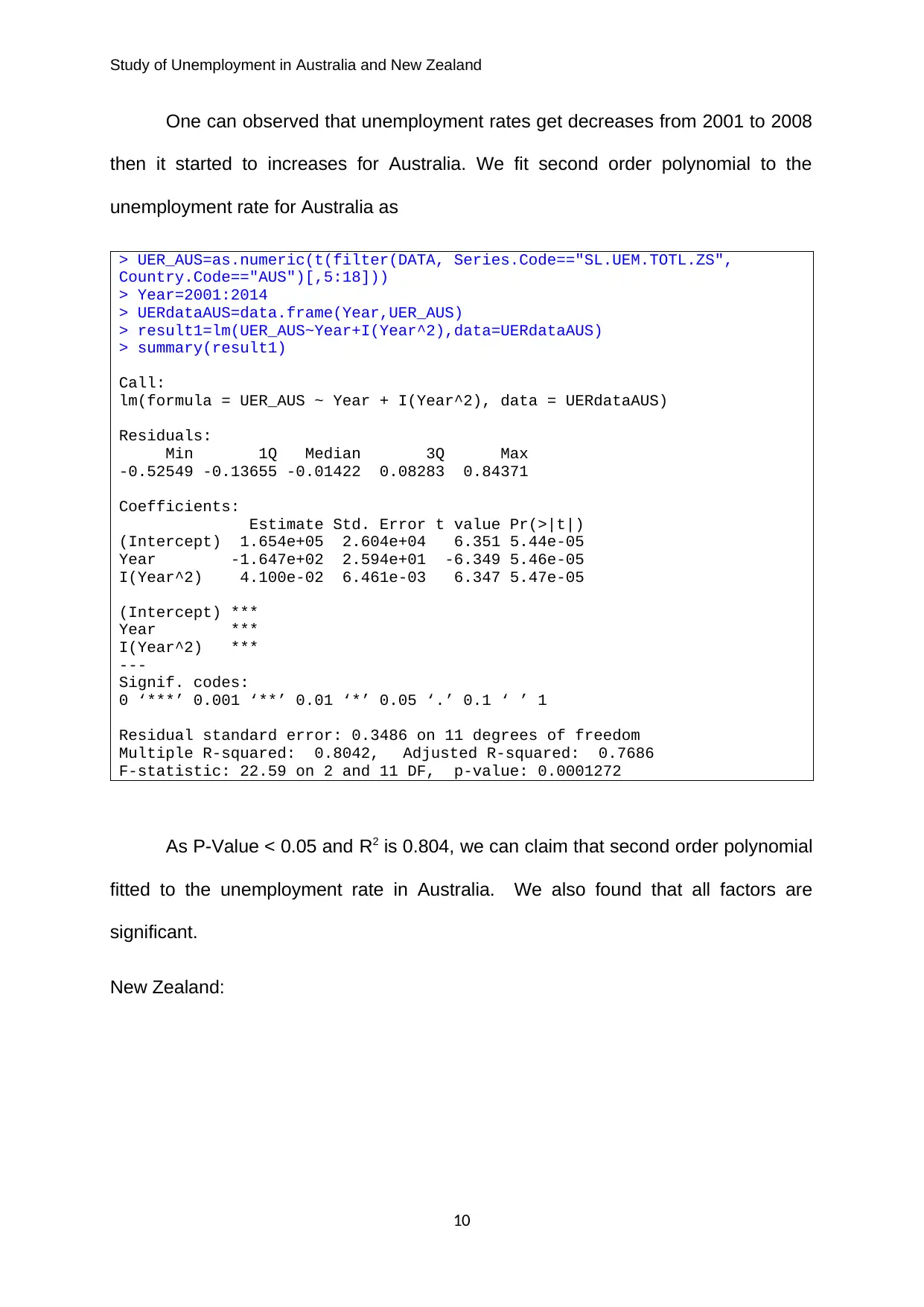
Data for unemployment rate is given for 2001 to 2014. We tried to fit line for
unemployment rate. We firstly plot the unemployment rate verses year to understand
the nature in Figure 5 and Figure 6 for Australia and New Zealand respectively.
Australia:
Figure 5: Unemployment rate for Australia from 2001 to 2014
9

Study of Unemployment in Australia and New Zealand
One can observed that unemployment rates get decreases from 2001 to 2008
then it started to increases for Australia. We fit second order polynomial to the
unemployment rate for Australia as
> UER_AUS=as.numeric(t(filter(DATA, Series.Code=="SL.UEM.TOTL.ZS",
Country.Code=="AUS")[,5:18]))
> Year=2001:2014
> UERdataAUS=data.frame(Year,UER_AUS)
> result1=lm(UER_AUS~Year+I(Year^2),data=UERdataAUS)
> summary(result1)
Call:
lm(formula = UER_AUS ~ Year + I(Year^2), data = UERdataAUS)
Residuals:
Min 1Q Median 3Q Max
-0.52549 -0.13655 -0.01422 0.08283 0.84371
Coefficients:
Estimate Std. Error t value Pr(>|t|)
(Intercept) 1.654e+05 2.604e+04 6.351 5.44e-05
Year -1.647e+02 2.594e+01 -6.349 5.46e-05
I(Year^2) 4.100e-02 6.461e-03 6.347 5.47e-05
(Intercept) ***
Year ***
I(Year^2) ***
---
Signif. codes:
0 ‘***’ 0.001 ‘**’ 0.01 ‘*’ 0.05 ‘.’ 0.1 ‘ ’ 1
Residual standard error: 0.3486 on 11 degrees of freedom
Multiple R-squared: 0.8042, Adjusted R-squared: 0.7686
F-statistic: 22.59 on 2 and 11 DF, p-value: 0.0001272
As P-Value < 0.05 and R2 is 0.804, we can claim that second order polynomial
fitted to the unemployment rate in Australia. We also found that all factors are
significant.
New Zealand:
10

Study of Unemployment in Australia and New Zealand
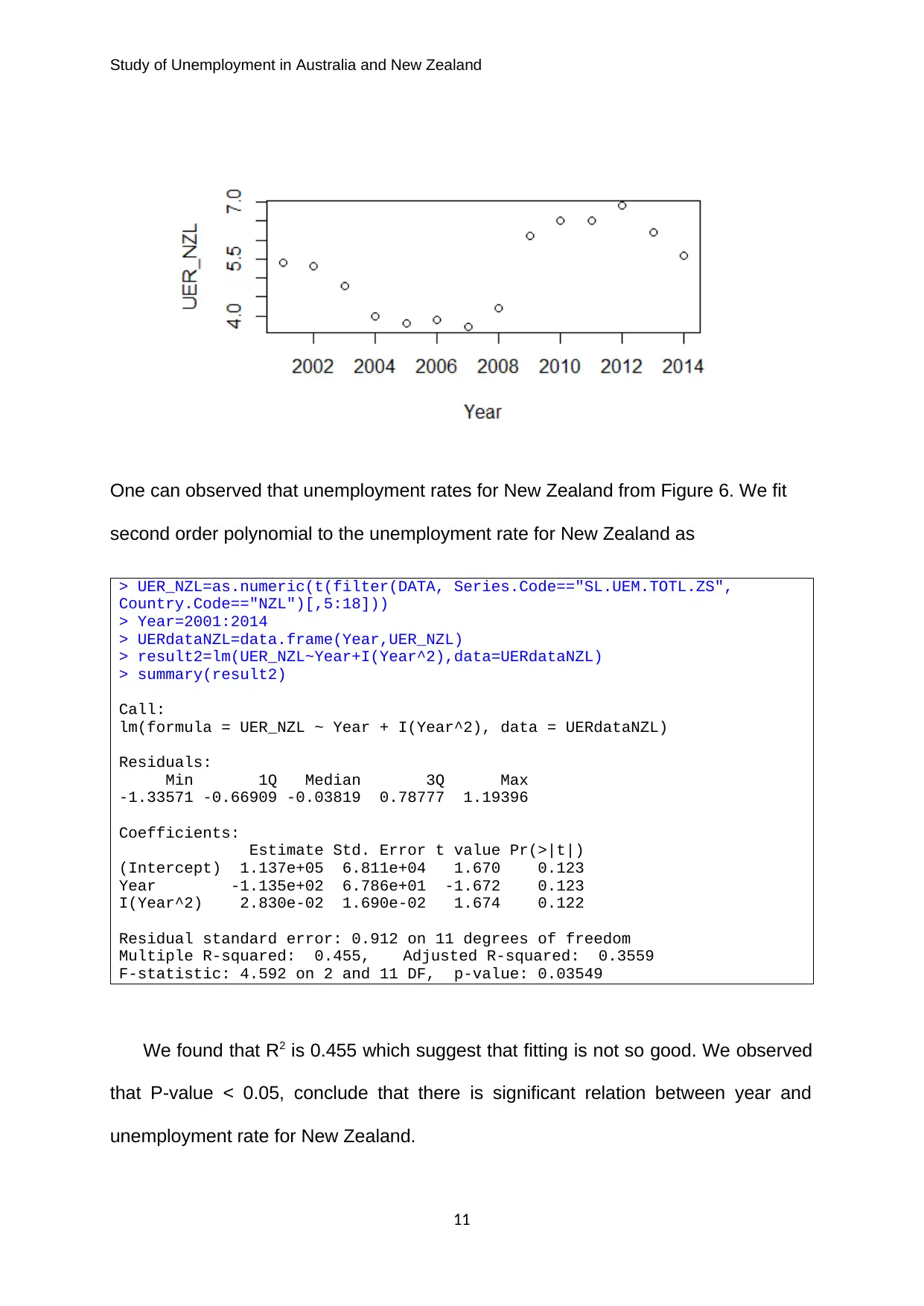
One can observed that unemployment rates for New Zealand from Figure 6. We fit
second order polynomial to the unemployment rate for New Zealand as
> UER_NZL=as.numeric(t(filter(DATA, Series.Code=="SL.UEM.TOTL.ZS",
Country.Code=="NZL")[,5:18]))
> Year=2001:2014
> UERdataNZL=data.frame(Year,UER_NZL)
> result2=lm(UER_NZL~Year+I(Year^2),data=UERdataNZL)
> summary(result2)
Call:
lm(formula = UER_NZL ~ Year + I(Year^2), data = UERdataNZL)
Residuals:
Min 1Q Median 3Q Max
-1.33571 -0.66909 -0.03819 0.78777 1.19396
Coefficients:
Estimate Std. Error t value Pr(>|t|)
(Intercept) 1.137e+05 6.811e+04 1.670 0.123
Year -1.135e+02 6.786e+01 -1.672 0.123
I(Year^2) 2.830e-02 1.690e-02 1.674 0.122
Residual standard error: 0.912 on 11 degrees of freedom
Multiple R-squared: 0.455, Adjusted R-squared: 0.3559
F-statistic: 4.592 on 2 and 11 DF, p-value: 0.03549
We found that R2 is 0.455 which suggest that fitting is not so good. We observed
that P-value < 0.05, conclude that there is significant relation between year and
unemployment rate for New Zealand.
11

Study of Unemployment in Australia and New Zealand
5. Conclusion
We observed that mean rate of unemployment is higher in Australia than New
Zealand whereas mean School enrollment, tertiary (% gross) is higher in New
Zealand than Australia. We reported that variation in unemployment rate for New
Zealand is higher than Australia whereas variation in school enrollment, tertiary (%
gross) for Australia is higher than New Zealand.
There is negative correlation between unemployment rate and school
enrollment, tertiary (% gross) for Australia whereas positive correlation between
unemployment rate and school enrollment, tertiary (% gross) for New Zealand.
We grouped the countries using clustering vector where 2: Low
Unemployment rate, 1: Medium Unemployment rate and 3: High employment Rate.
We observed that Australia and New Zealand are in high unemployment group.
We fitted second order polynomial to the unemployment rate in Australia and
found suitable. We also found that all factors are significant. We observed that there
is significant relation between year and unemployment rate for New Zealand.
6. Reflection
Data filter and handling of not available values of variables of interest is main
problem in this analysis. We used filter function defined in dplyr library for filtering
data and na.omit function to omit the not available values. We got the interest after
getting desired data in desired format. By doing this study, we got the confidence on
the handling the big data analysis.
12

Study of Unemployment in Australia and New Zealand
List of References
Anderberg, M.R., 2014. Cluster analysis for applications: probability and
mathematical statistics: a series of monographs and textbooks (Vol. 19).
Academic press.
Baayen, R.H., 2008. Analyzing linguistic data: A practical introduction to statistics
using R. Cambridge University Press.
Berenson, M., Levine, D., Szabat, K.A. and Krehbiel, T.C., 2012. Basic business
statistics: Concepts and applications. Pearson higher education AU.
Bickel, P.J. and Doksum, K.A., 2015. Mathematical statistics: basic ideas and
selected topics, volume I (Vol. 117). CRC Press.
Casella, G. and Berger, R.L., 2002. Statistical inference (Vol. 2). Pacific Grove, CA:
Duxbury.
DeGroot, M.H. and Schervish, M.J., 2012. Probability and statistics. Pearson
Education.
Devore, J.L. and Berk, K.N., 2007. Modern mathematical statistics with applications.
Cengage Learning.
Groebner, D.F., Shannon, P.W., Fry, P.C. and Smith, K.D., 2008. Business statistics.
Pearson Education.
Hair, J.F., Black, W.C., Babin, B.J., Anderson, R.E. and Tatham, R.L.,
1998. Multivariate data analysis (Vol. 5, No. 3, pp. 207-219). Upper Saddle
River, NJ: Prentice hall.
Hoel, P.G., 1954. Introduction to mathematical statistics. Introduction to
mathematical statistics., (2nd Ed).
Hogg, R.V. and Craig, A.T., 1995. Introduction to mathematical statistics.(5"" edition)
(pp. 269-278). Upper Saddle River, New Jersey: Prentice Hall.
Hopkins, K.D., Glass, G.V. and Hopkins, B.R., 1987. Basic statistics for the
behavioral sciences. Prentice-Hall, Inc.
13

Study of Unemployment in Australia and New Zealand
Kaufman, L. and Rousseeuw, P.J., 2009. Finding groups in data: an introduction to
cluster analysis (Vol. 344). John Wiley & Sons.
Larsen, R.J. and Marx, M.L., 2017. An introduction to mathematical statistics and its
applications (Vol. 5). Pearson.
Romesburg, C., 2004. Cluster analysis for researchers. Lulu. com.
Ross, S.M., 2014. Introduction to probability models. Academic press.
Serfling, R.J., 2009. Approximation theorems of mathematical statistics (Vol. 162).
John Wiley & Sons.
14