Univariate Analysis II Regression

UNIVARIATE ANALYSIS II: REGRESSION
Student Name:
Instructor Name:
Course Number:
20th February 2020

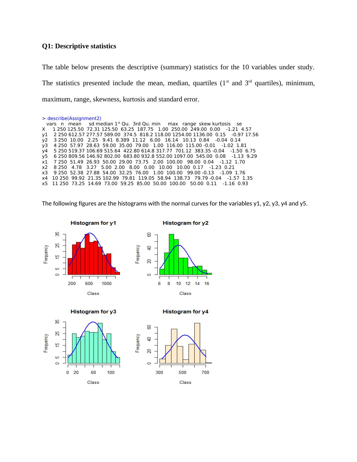
Q1: Descriptive statistics
The table below presents the descriptive (summary) statistics for the 10 variables under study.
The statistics presented include the mean, median, quartiles (1st and 3rd quartiles), minimum,
maximum, range, skewness, kurtosis and standard error.
> describe(Assignment2)
vars n mean sd median 1st Qu. 3rd Qu. min max range skew kurtosis se
X 1 250 125.50 72.31 125.50 63.25 187.75 1.00 250.00 249.00 0.00 -1.21 4.57
y1 2 250 612.57 277.57 589.00 374.5 818.2 118.00 1254.00 1136.00 0.15 -0.97 17.56
y2 3 250 10.00 2.25 9.41 8.389 11.12 6.00 16.14 10.13 0.84 -0.04 0.14
y3 4 250 57.97 28.63 59.00 35.00 79.00 1.00 116.00 115.00 -0.01 -1.02 1.81
y4 5 250 519.37 106.69 515.64 422.80 614.8 317.77 701.12 383.35 -0.04 -1.50 6.75
y5 6 250 809.56 146.92 802.00 683.80 932.8 552.00 1097.00 545.00 0.08 -1.13 9.29
x1 7 250 51.49 26.93 50.00 29.00 73.75 2.00 100.00 98.00 0.04 -1.12 1.70
x2 8 250 4.78 3.27 5.00 2.00 8.00 0.00 10.00 10.00 0.17 -1.23 0.21
x3 9 250 52.38 27.88 54.00 32.25 76.00 1.00 100.00 99.00 -0.13 -1.09 1.76
x4 10 250 99.92 21.35 102.99 79.81 119.05 58.94 138.73 79.79 -0.04 -1.57 1.35
x5 11 250 73.25 14.69 73.00 59.25 85.00 50.00 100.00 50.00 0.11 -1.16 0.93
The following figures are the histograms with the normal curves for the variables y1,
y2, y3, y4 and y5.

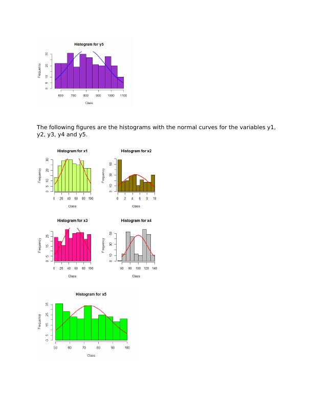
The following figures are the histograms with the normal curves for the variables y1,
y2, y3, y4 and y5.

Q2 : Residual diagnostics
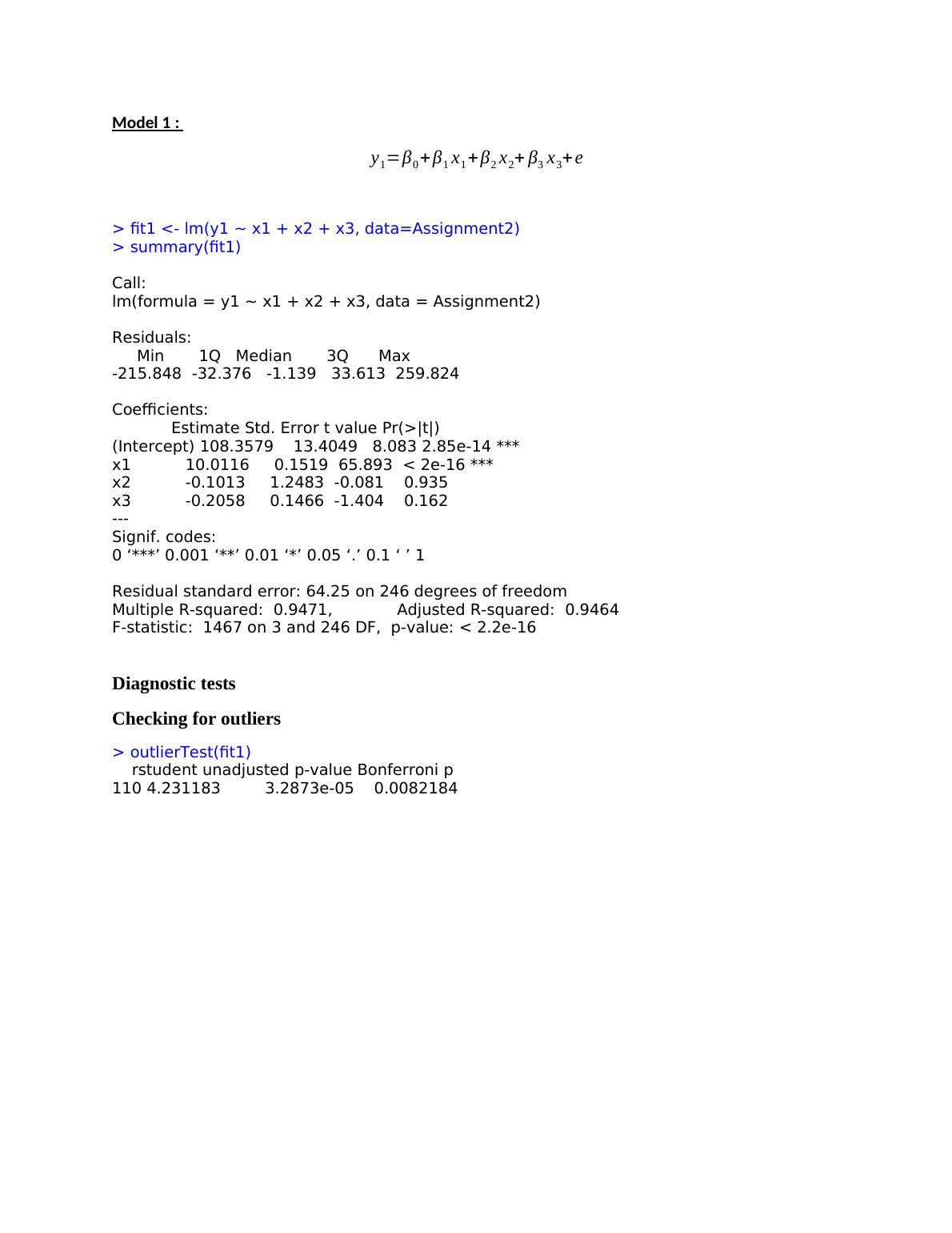
Model 1 :
y1=β0 + β1 x1 + β2 x2+ β3 x3+ e
> fit1 <- lm(y1 ~ x1 + x2 + x3, data=Assignment2)
> summary(fit1)
Call:
lm(formula = y1 ~ x1 + x2 + x3, data = Assignment2)
Residuals:
Min 1Q Median 3Q Max
-215.848 -32.376 -1.139 33.613 259.824
Coefficients:
Estimate Std. Error t value Pr(>|t|)
(Intercept) 108.3579 13.4049 8.083 2.85e-14 ***
x1 10.0116 0.1519 65.893 < 2e-16 ***
x2 -0.1013 1.2483 -0.081 0.935
x3 -0.2058 0.1466 -1.404 0.162
---
Signif. codes:
0 ‘***’ 0.001 ‘**’ 0.01 ‘*’ 0.05 ‘.’ 0.1 ‘ ’ 1
Residual standard error: 64.25 on 246 degrees of freedom
Multiple R-squared: 0.9471, Adjusted R-squared: 0.9464
F-statistic: 1467 on 3 and 246 DF, p-value: < 2.2e-16
Diagnostic tests
Checking for outliers
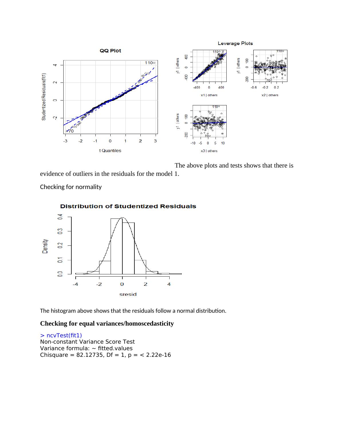
> outlierTest(fit1)
rstudent unadjusted p-value Bonferroni p
110 4.231183 3.2873e-05 0.0082184

The above plots and tests shows that there is
evidence of outliers in the residuals for the model 1.
Checking for normality
The histogram above shows that the residuals follow a normal distribution.
Checking for equal variances/homoscedasticity
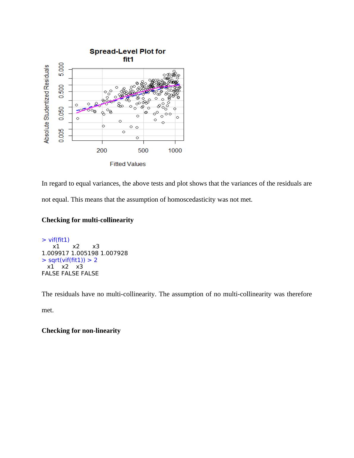
> ncvTest(fit1)
Non-constant Variance Score Test
Variance formula: ~ fitted.values
Chisquare = 82.12735, Df = 1, p = < 2.22e-16

In regard to equal variances, the above tests and plot shows that the variances of the residuals are
not equal. This means that the assumption of homoscedasticity was not met.
Checking for multi-collinearity
> vif(fit1)
x1 x2 x3
1.009917 1.005198 1.007928
> sqrt(vif(fit1)) > 2
x1 x2 x3
FALSE FALSE FALSE
The residuals have no multi-collinearity. The assumption of no multi-collinearity was therefore
met.
Checking for non-linearity