STAT2000 Quantitative Analysis: Statistical Evaluation of Data

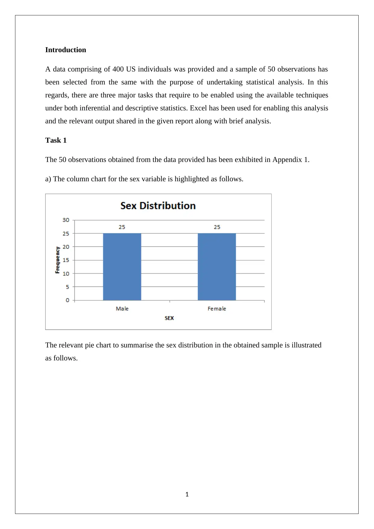
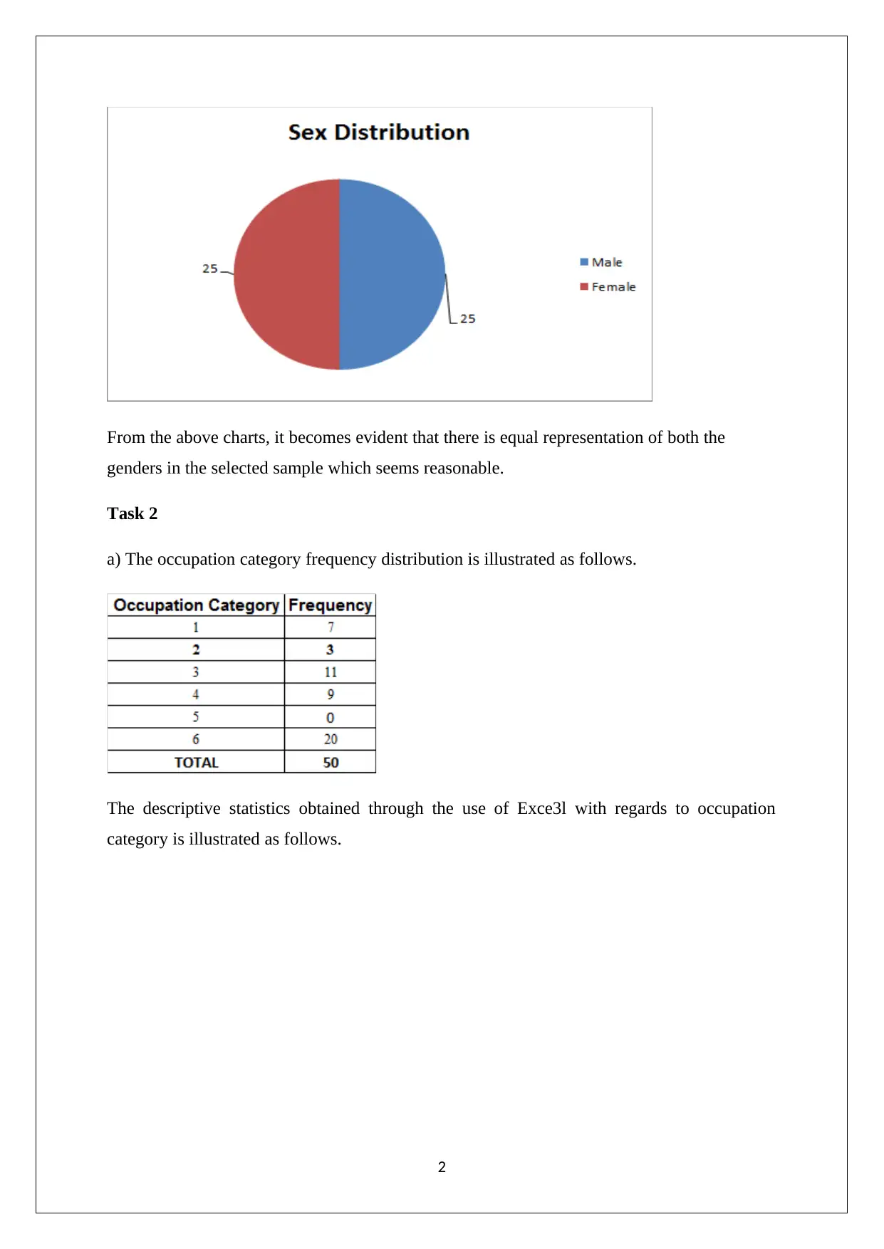
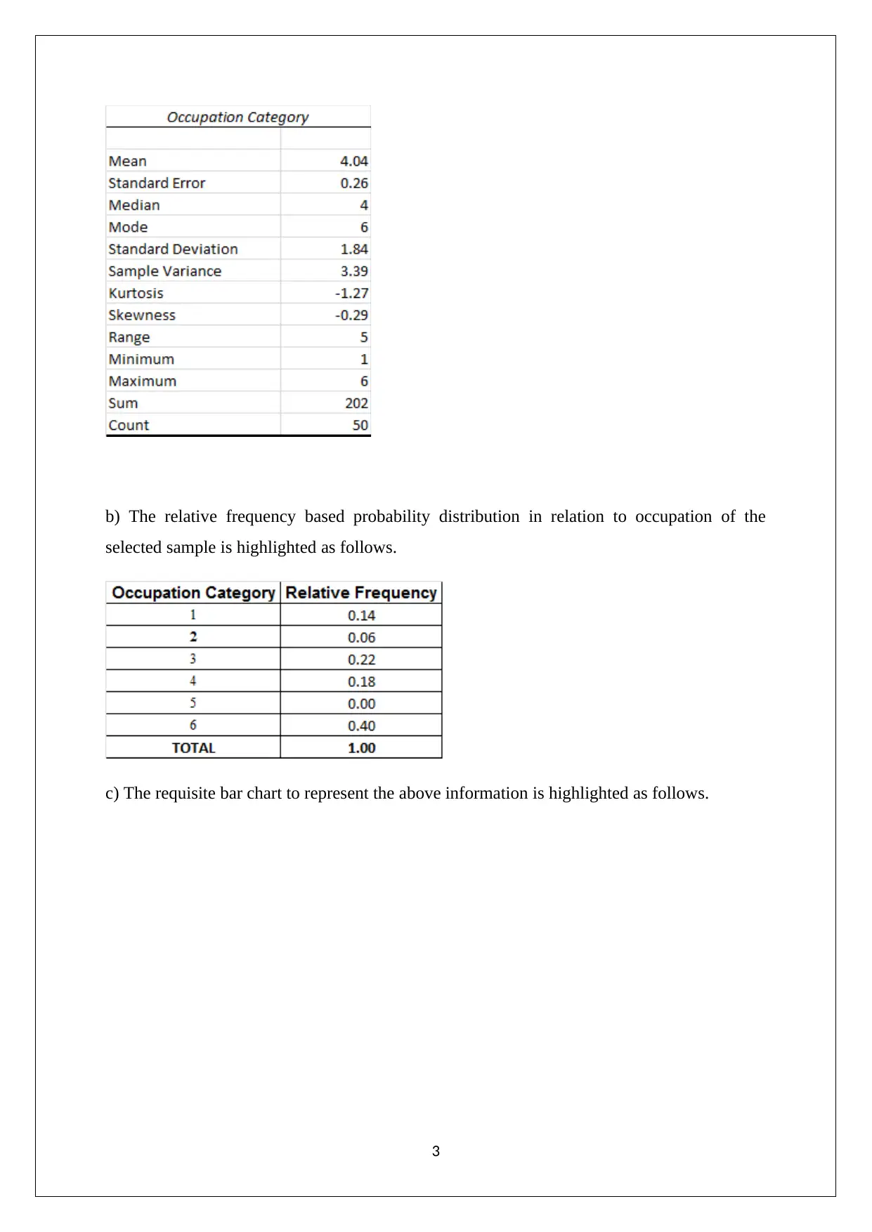
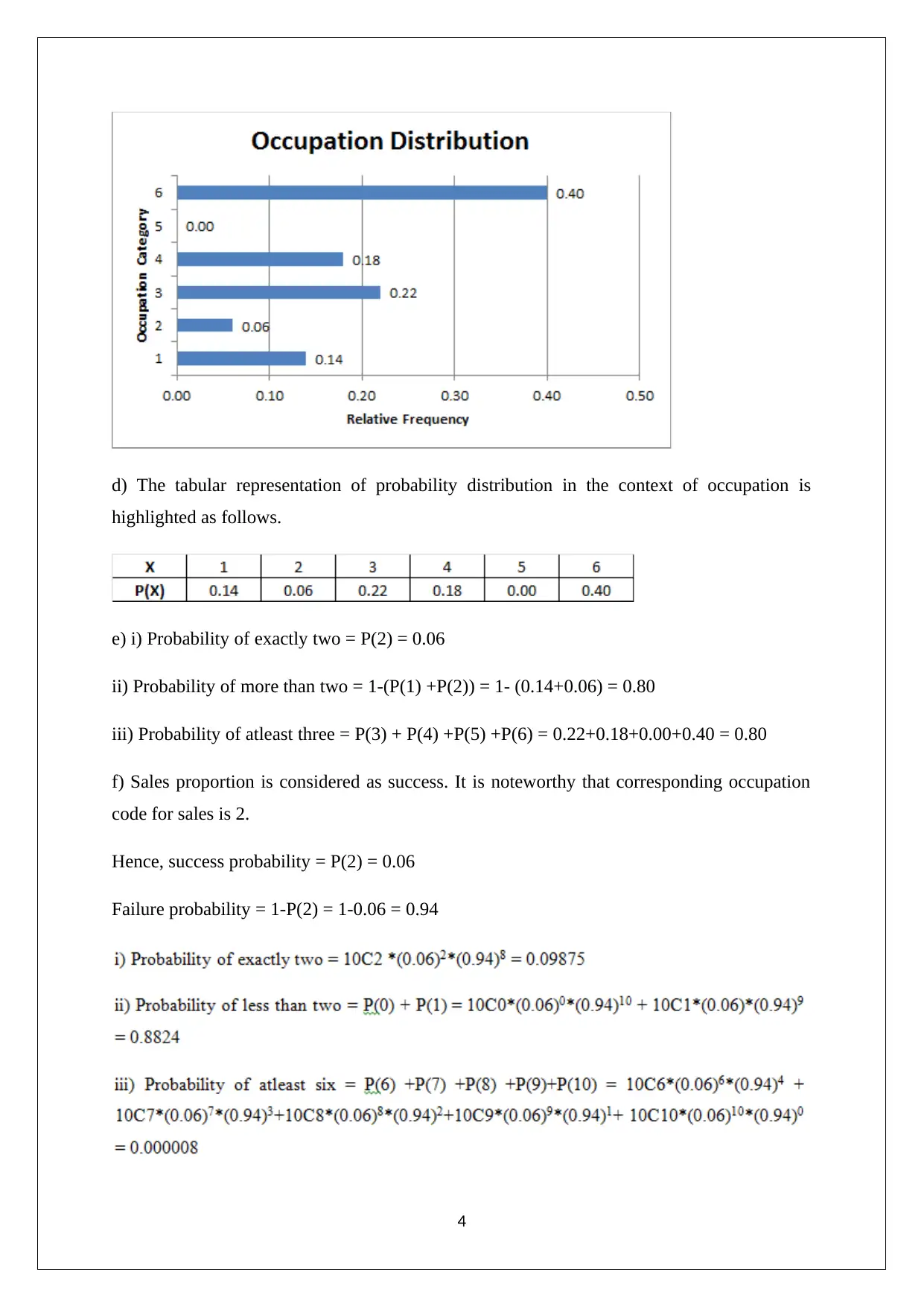
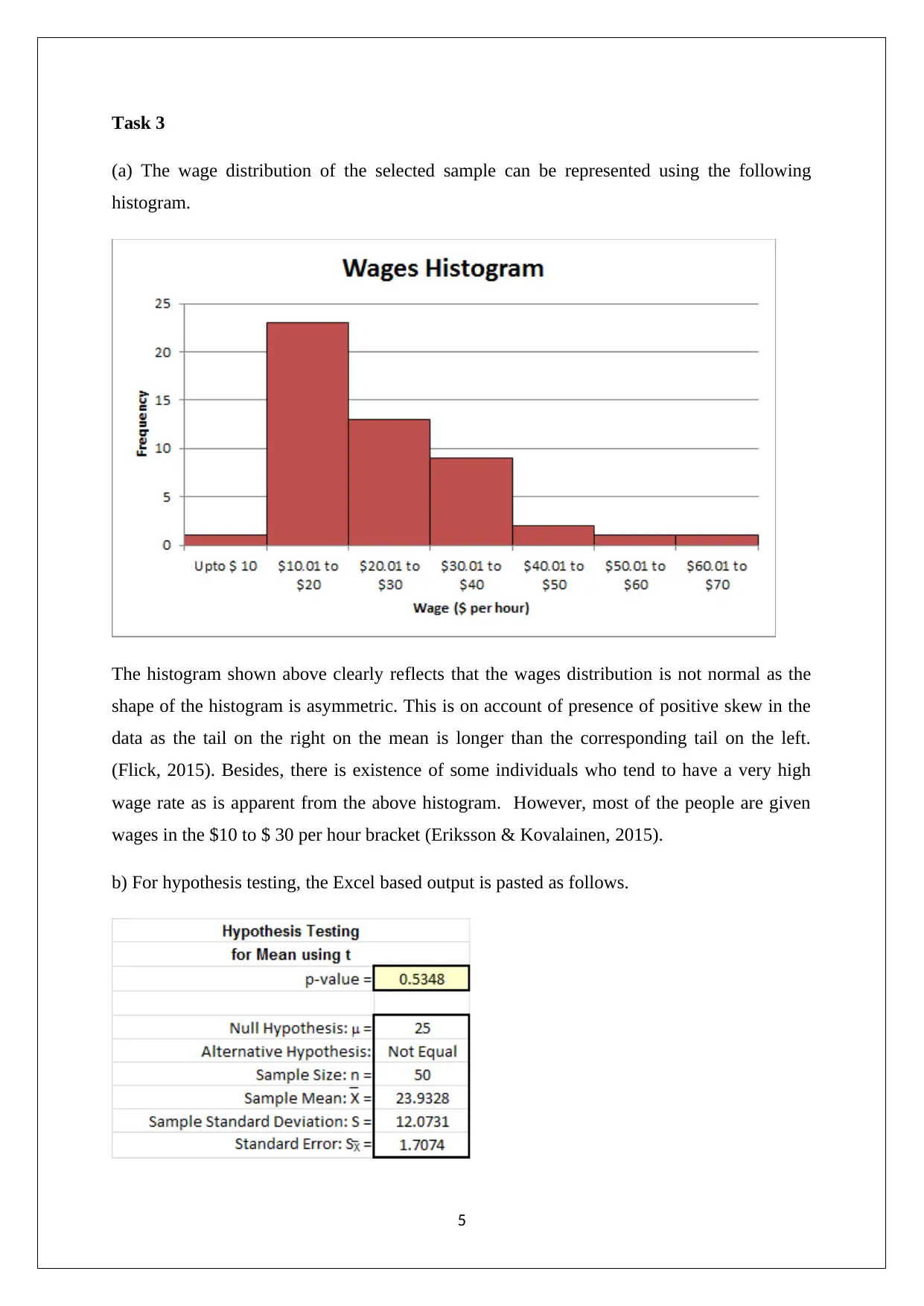
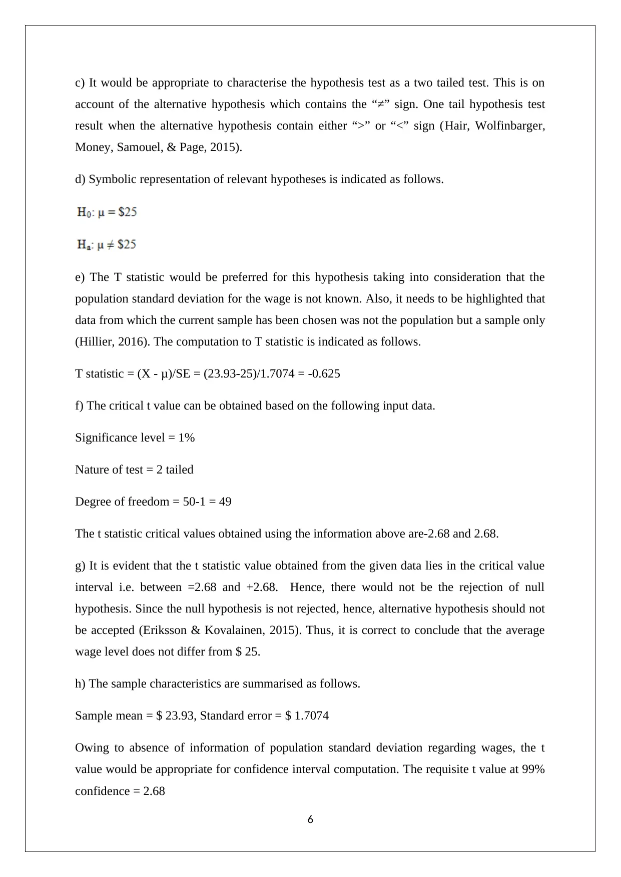
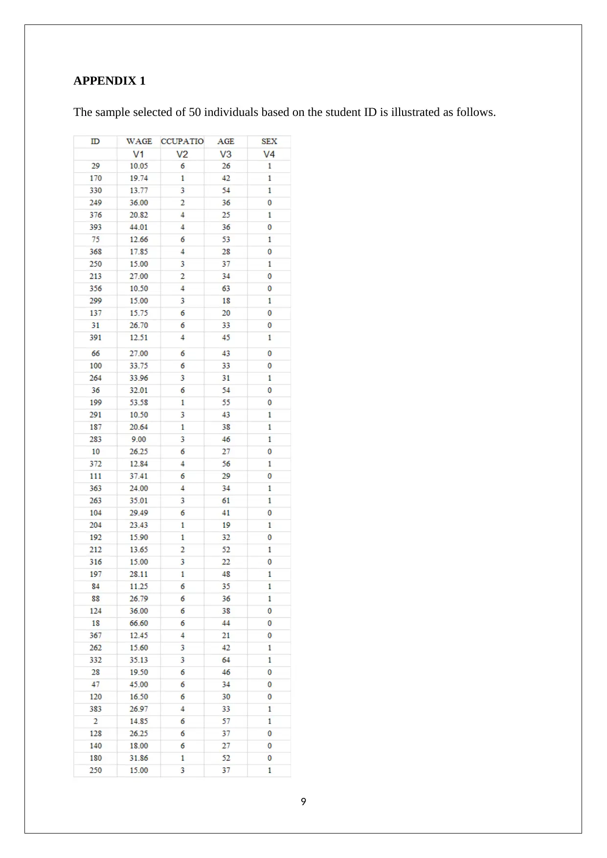
This report presents a quantitative analysis of a dataset comprising 400 US individuals, with a sample of 50 observations selected for statistical analysis. The analysis encompasses three major tasks using techniques under both inferential and descriptive statistics, enabled by Excel. The report includes ...Read More

STAT2000-Quantitative Analysis
STUDENT ID:
[Pick the date]

Introduction
A data comprising of 400 US individuals was provided and a sample of 50 observations has
been selected from the same with the purpose of undertaking statistical analysis. In this
regards, there are three major tasks that require to be enabled using the available techniques
under both inferential and descriptive statistics. Excel has been used for enabling this analysis
and the relevant output shared in the given report along with brief analysis.
Task 1
The 50 observations obtained from the data provided has been exhibited in Appendix 1.
a) The column chart for the sex variable is highlighted as follows.
The relevant pie chart to summarise the sex distribution in the obtained sample is illustrated
as follows.
1

From the above charts, it becomes evident that there is equal representation of both the
genders in the selected sample which seems reasonable.
Task 2
a) The occupation category frequency distribution is illustrated as follows.
The descriptive statistics obtained through the use of Exce3l with regards to occupation
category is illustrated as follows.
2

b) The relative frequency based probability distribution in relation to occupation of the
selected sample is highlighted as follows.
c) The requisite bar chart to represent the above information is highlighted as follows.
3

d) The tabular representation of probability distribution in the context of occupation is
highlighted as follows.
e) i) Probability of exactly two = P(2) = 0.06
ii) Probability of more than two = 1-(P(1) +P(2)) = 1- (0.14+0.06) = 0.80
iii) Probability of atleast three = P(3) + P(4) +P(5) +P(6) = 0.22+0.18+0.00+0.40 = 0.80
f) Sales proportion is considered as success. It is noteworthy that corresponding occupation
code for sales is 2.
Hence, success probability = P(2) = 0.06
Failure probability = 1-P(2) = 1-0.06 = 0.94
4

Task 3
(a) The wage distribution of the selected sample can be represented using the following
histogram.
The histogram shown above clearly reflects that the wages distribution is not normal as the
shape of the histogram is asymmetric. This is on account of presence of positive skew in the
data as the tail on the right on the mean is longer than the corresponding tail on the left.
(Flick, 2015). Besides, there is existence of some individuals who tend to have a very high
wage rate as is apparent from the above histogram. However, most of the people are given
wages in the $10 to $ 30 per hour bracket (Eriksson & Kovalainen, 2015).
b) For hypothesis testing, the Excel based output is pasted as follows.
5

c) It would be appropriate to characterise the hypothesis test as a two tailed test. This is on
account of the alternative hypothesis which contains the “≠” sign. One tail hypothesis test
result when the alternative hypothesis contain either “>” or “<” sign (Hair, Wolfinbarger,
Money, Samouel, & Page, 2015).
d) Symbolic representation of relevant hypotheses is indicated as follows.
e) The T statistic would be preferred for this hypothesis taking into consideration that the
population standard deviation for the wage is not known. Also, it needs to be highlighted that
data from which the current sample has been chosen was not the population but a sample only
(Hillier, 2016). The computation to T statistic is indicated as follows.
T statistic = (X - μ)/SE = (23.93-25)/1.7074 = -0.625
f) The critical t value can be obtained based on the following input data.
Significance level = 1%
Nature of test = 2 tailed
Degree of freedom = 50-1 = 49
The t statistic critical values obtained using the information above are-2.68 and 2.68.
g) It is evident that the t statistic value obtained from the given data lies in the critical value
interval i.e. between =2.68 and +2.68. Hence, there would not be the rejection of null
hypothesis. Since the null hypothesis is not rejected, hence, alternative hypothesis should not
be accepted (Eriksson & Kovalainen, 2015). Thus, it is correct to conclude that the average
wage level does not differ from $ 25.
h) The sample characteristics are summarised as follows.
Sample mean = $ 23.93, Standard error = $ 1.7074
Owing to absence of information of population standard deviation regarding wages, the t
value would be appropriate for confidence interval computation. The requisite t value at 99%
confidence = 2.68
6

Upper level of 99% confidence interval for mean wage = 23.93 + 2.68*1.7074 = $ 28.51
Lower level of 99% confidence interval for mean wage = 23.93 - 2.68*1.7074 = $ 19.36
i) In the given case, there has been a change in confidence level which has become 95% and
therefore a change in the critical values would be initiated. While this would not alter the
computation of t statistic but the critical value would get changed to -2.01 and 2.01 (Flick,
2015)
j) It is evident that the t statistic value obtained from the given data lies in the critical value
interval i.e. between =2.01 and +2.01. Hence, there would not be the rejection of null
hypothesis. Since the null hypothesis is not rejected, hence, alternative hypothesis should not
be accepted (Eriksson & Kovalainen, 2015). Thus, it is correct to conclude that the average
wage level does not differ from $ 25.
k) The sample characteristics are summarised as follows.
Sample mean = $ 23.93, Standard error = $ 1.7074
Owing to absence of information of population standard deviation regarding wages, the t
value would be appropriate for confidence interval computation. The requisite t value at 95%
confidence = 2.01
l) Based on the 9% confidence interval, it may be concluded that a 95% probability exists that
the population average wage would fall in the ($ 20.50, $27.36) interval. Additionally, it is
evident when the two confidence intervals are compared that higher precision in estimation of
population mean typically leads to confidence interval that is wider (Hillier, 2016).
Conclusion
The probability distribution of various occupations has been derived indicating that there is
no professional in the selected sample. The gender distribution is fair as both sex have equal
representation. Also, the distribution of wage is not normal owing to presence of some highly
paid individuals. Besides, based on testing of hypothesis at 1% and 5% significance level, the
population average wage does not seem to deviate from $ 25 per hour.
7

References
Eriksson, P. & Kovalainen, A. (2015) Quantitative methods in business research. 3rd ed.
London: Sage Publications.
Flick, U. (2015) Introducing research methodology: A beginner's guide to doing a research
project. 4th ed. New York: Sage Publications
Hair, J. F., Wolfinbarger, M., Money, A. H., Samouel, P., & Page, M. J. (2015) Essentials of
business research methods. 2nd ed. New York: Routledge.
Hillier, F. (2016) Introduction to Operations Research. 6th ed. New York: McGraw Hill
Publications.
8

APPENDIX 1
The sample selected of 50 individuals based on the student ID is illustrated as follows.
9