Understanding Volatility, Standard Deviation, and Risk in Finance

This article explains the concepts of volatility, standard deviation, and risk in finance. It clarifies the differences between these terms and their significance in financial modeling and forecasting. The article also discusses the complexities involved in estimating volatility and forecasting results. Desklib provides access to solved assignments, essays, and dissertations on this topic.

Dear tutor,
This is the paraphrasing task to replace my failure assignment made earlier No.
The only task to do is paraphrasing the text in the paraphrasing section in Red color.
Please don't change terminologies , for example: standard deviation, normal distribution etc.
Regards
References Text Paraphrasing section
Volatility
Term & Concept
Many investors and generations of finance students often
have an incomplete appreciation of the differences between
volatility, standard deviation, and risk. It is worth elucidating
some of the conceptual issues here. In finance, volatility is
often used to refer to standard deviation, σ, or variance, σ2,
Term and Concept
Numerous students of finance and investors have analysed contrasts
between standard deviation, variation and risk. It merits clarifying a
portion of the reasonable issues here. In fund, volatility is frequently
used to allude to standard deviation, σ, or variance, σ2, computed as:

Definition
(Poon &
Granger, 2003)
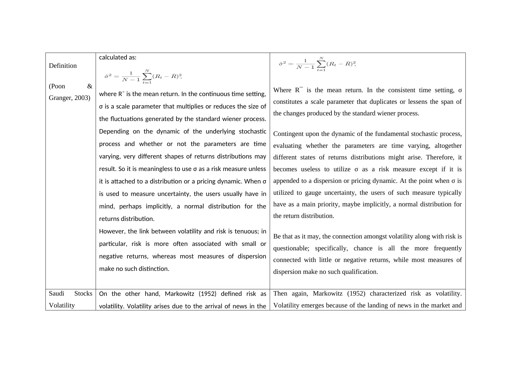
calculated as:
where R¯ is the mean return. In the continuous time setting,
σ is a scale parameter that multiplies or reduces the size of
the fluctuations generated by the standard wiener process.
Depending on the dynamic of the underlying stochastic
process and whether or not the parameters are time
varying, very different shapes of returns distributions may
result. So it is meaningless to use σ as a risk measure unless
it is attached to a distribution or a pricing dynamic. When σ
is used to measure uncertainty, the users usually have in
mind, perhaps implicitly, a normal distribution for the
returns distribution.
However, the link between volatility and risk is tenuous; in
particular, risk is more often associated with small or
negative returns, whereas most measures of dispersion
make no such distinction.
Where R¯ is the mean return. In the consistent time setting, σ
constitutes a scale parameter that duplicates or lessens the span of
the changes produced by the standard wiener process.
Contingent upon the dynamic of the fundamental stochastic process,
evaluating whether the parameters are time varying, altogether
different states of returns distributions might arise. Therefore, it
becomes useless to utilize σ as a risk measure except if it is
appended to a dispersion or pricing dynamic. At the point when σ is
utilized to gauge uncertainty, the users of such measure typically
have as a main priority, maybe implicitly, a normal distribution for
the return distribution.
Be that as it may, the connection amongst volatility along with risk is
questionable; specifically, chance is all the more frequently
connected with little or negative returns, while most measures of
dispersion make no such qualification.
Saudi Stocks
Volatility
On the other hand, Markowitz (1952) defined risk as
volatility. Volatility arises due to the arrival of news in the
Then again, Markowitz (1952) characterized risk as volatility.
Volatility emerges because of the landing of news in the market and

(Kalyanaraman
, 2014)
market and the consequent trading activity by the traders.
Dispersion of beliefs among the traders will cause a rise in
the level of volatility. When volatility is high compared to
the equilibrium values of the stocks, it impacts the return on
the stock investment.
the subsequent exchanging action by the brokers. Scattering of
convictions among the merchants will cause a rise in the level of
volatility. At the point when volatility is high contrasted with the
balance estimations of the stocks, it impacts the arrival on the stock
speculation.
Volatility
Definition
(Poon &
Granger, 2003)
Concept & Definition:
In general terms, volatility refers to the fluctuations
observed in some phenomenon over time. In terms of
modelling and forecasting literature, it means “the
conditional variance of the underlying asset return” (Tsay,
2010).
From the previous discussion, volatility is often calculated as
the sample standard deviation, which is the square root of
the equation. Stephen Figlewski (1997) notes that since the
statistical properties of sample mean make it a very
inaccurate estimate of the true mean, especially for small
samples, taking deviations around zero instead of the
sample mean as in equation typically increases volatility
forecast accuracy. There are methods for estimating
volatility that are designed to exploit or reduce the
Concepts and Definition:
Volatility, generally alludes to the fluctuations noted for some
phenomenon for a period of time. Regarding modeling and
forecasting literature, it signifies "the conditional variance of the
underlying asset return" (Tsay, 2010).
From the past argument, volatility is regularly computed as the
sample standard deviation, which is the square foundation of the
condition. Stephen Figlewski (1997) provides that since the
statistical properties of sample mean make it an extremely inaccurate
estimate of the true mean, particularly for smaller size samples,
taking deviations around zero rather than the sample mean as in
condition normally expands volatility conjecture precision. There are
techniques for assessing volatility that are intended to misuse or
lessen the impact of extremes. While past condition (1) is a fair

influence of extremes. While previous equation (1) is an
unbiased estimate of σ2, the square root of σˆ2 is a biased
estimate of σ due to Jensen inequality. Ding et al (1993)
suggest measuring volatility directly from absolute returns.
Marie Davidian and Raymond Carroll (1987) show absolute
returns volatility specification is more robust against
asymmetry and non-normality. There is some empirical
evidence that deviations or absolute returns based models
produce better volatility forecasts than models based on
squared returns (Stephen Taylor 1986; Louis Ederinton and
Wei Guan 2000a; and Michael McKenzie 1999) but the
majority of time series volatility models are squared returns
models.
Time Series & stylized fact:
There are several salient features about financial time series
and financial market volatility that are now well
documented. These include fat tail distributions of risky
asset returns, volatility clustering, asymmetry and mean
reversion, and co-movements of volatilities across assets
and financial markets.
gauge of σ2, the square base of σˆ2 is a one-sided gauge of σ because
of Jensen disparity. Ding et al (1993) propose estimating volatility
specifically from total returns. Marie Davidian and Raymond Carroll
(1987) indicate absolute returns volatility determination is more
powerful against asymmetry and non-normality. There is some
experimental confirmation that deviations or supreme returns based
models deliver preferable volatility estimates over models in view of
squared returns (Stephen Taylor 1986; Louis Ederinton and Wei
Guan 2000a; and Michael McKenzie 1999) yet most of time series
volatility models are squared returns models.
Time Series and adapted reality:
There are a few notable highlights about financial time arrangement
and financial related market volatility that are presently very much
reported. These incorporate fat tail circulations of risky asset returns,
volatility clustering, asymmetry and mean reversion and co-
movements of volatilities over assets and financial markets.
Since volatility of financial time arrangement has complex structure,

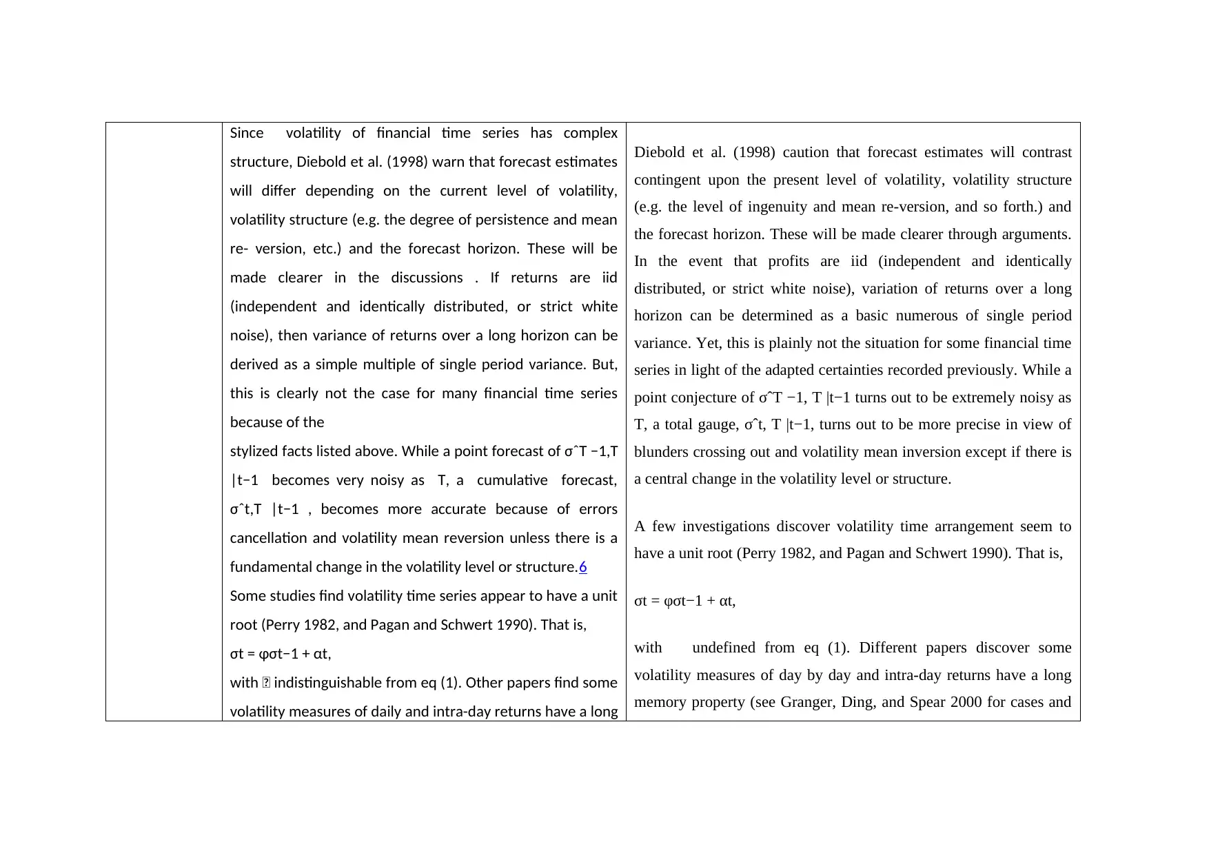
Since volatility of financial time series has complex
structure, Diebold et al. (1998) warn that forecast estimates
will differ depending on the current level of volatility,
volatility structure (e.g. the degree of persistence and mean
re- version, etc.) and the forecast horizon. These will be
made clearer in the discussions . If returns are iid
(independent and identically distributed, or strict white
noise), then variance of returns over a long horizon can be
derived as a simple multiple of single period variance. But,
this is clearly not the case for many financial time series
because of the
stylized facts listed above. While a point forecast of σˆT −1,T
|t−1 becomes very noisy as T, a cumulative forecast,
σˆt,T |t−1 , becomes more accurate because of errors
cancellation and volatility mean reversion unless there is a
fundamental change in the volatility level or structure.6
Some studies find volatility time series appear to have a unit
root (Perry 1982, and Pagan and Schwert 1990). That is,
σt = φσt−1 + αt,
with  indistinguishable from eq (1). Other papers find some
volatility measures of daily and intra-day returns have a long
Diebold et al. (1998) caution that forecast estimates will contrast
contingent upon the present level of volatility, volatility structure
(e.g. the level of ingenuity and mean re-version, and so forth.) and
the forecast horizon. These will be made clearer through arguments.
In the event that profits are iid (independent and identically
distributed, or strict white noise), variation of returns over a long
horizon can be determined as a basic numerous of single period
variance. Yet, this is plainly not the situation for some financial time
series in light of the adapted certainties recorded previously. While a
point conjecture of σˆT −1, T |t−1 turns out to be extremely noisy as
T, a total gauge, σˆt, T |t−1, turns out to be more precise in view of
blunders crossing out and volatility mean inversion except if there is
a central change in the volatility level or structure.
A few investigations discover volatility time arrangement seem to
have a unit root (Perry 1982, and Pagan and Schwert 1990). That is,
σt = φσt−1 + αt,
with  undefined from eq (1). Different papers discover some
volatility measures of day by day and intra-day returns have a long
memory property (see Granger, Ding, and Spear 2000 for cases and

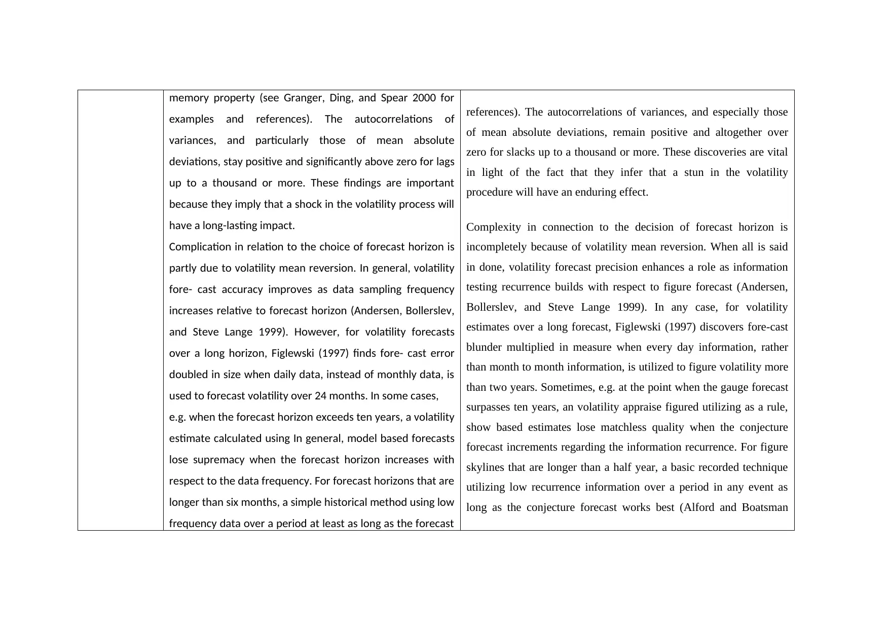
memory property (see Granger, Ding, and Spear 2000 for
examples and references). The autocorrelations of
variances, and particularly those of mean absolute
deviations, stay positive and significantly above zero for lags
up to a thousand or more. These findings are important
because they imply that a shock in the volatility process will
have a long-lasting impact.
Complication in relation to the choice of forecast horizon is
partly due to volatility mean reversion. In general, volatility
fore- cast accuracy improves as data sampling frequency
increases relative to forecast horizon (Andersen, Bollerslev,
and Steve Lange 1999). However, for volatility forecasts
over a long horizon, Figlewski (1997) finds fore- cast error
doubled in size when daily data, instead of monthly data, is
used to forecast volatility over 24 months. In some cases,
e.g. when the forecast horizon exceeds ten years, a volatility
estimate calculated using In general, model based forecasts
lose supremacy when the forecast horizon increases with
respect to the data frequency. For forecast horizons that are
longer than six months, a simple historical method using low
frequency data over a period at least as long as the forecast
references). The autocorrelations of variances, and especially those
of mean absolute deviations, remain positive and altogether over
zero for slacks up to a thousand or more. These discoveries are vital
in light of the fact that they infer that a stun in the volatility
procedure will have an enduring effect.
Complexity in connection to the decision of forecast horizon is
incompletely because of volatility mean reversion. When all is said
in done, volatility forecast precision enhances a role as information
testing recurrence builds with respect to figure forecast (Andersen,
Bollerslev, and Steve Lange 1999). In any case, for volatility
estimates over a long forecast, Figlewski (1997) discovers fore-cast
blunder multiplied in measure when every day information, rather
than month to month information, is utilized to figure volatility more
than two years. Sometimes, e.g. at the point when the gauge forecast
surpasses ten years, an volatility appraise figured utilizing as a rule,
show based estimates lose matchless quality when the conjecture
forecast increments regarding the information recurrence. For figure
skylines that are longer than a half year, a basic recorded technique
utilizing low recurrence information over a period in any event as
long as the conjecture forecast works best (Alford and Boatsman

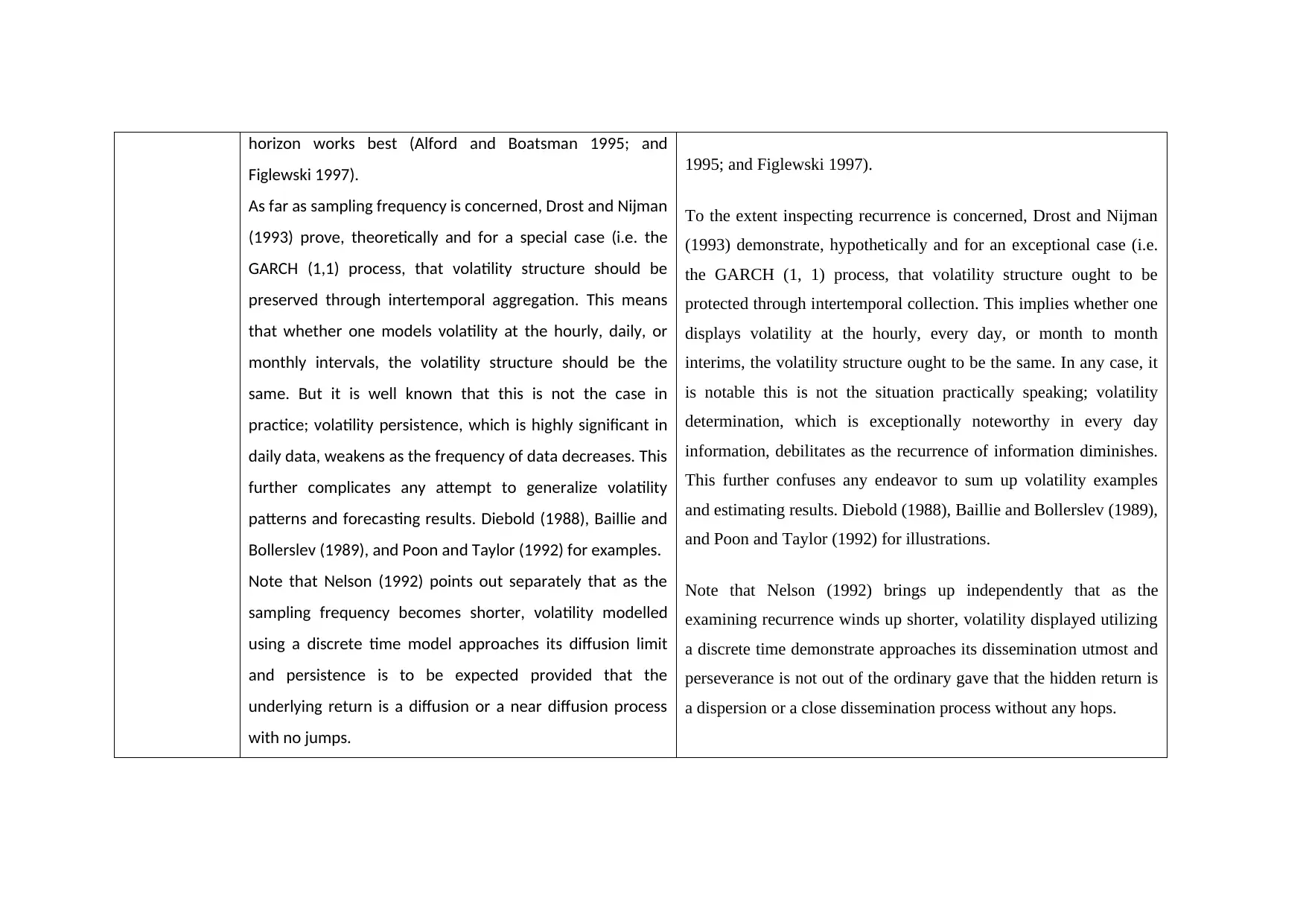
horizon works best (Alford and Boatsman 1995; and
Figlewski 1997).
As far as sampling frequency is concerned, Drost and Nijman
(1993) prove, theoretically and for a special case (i.e. the
GARCH (1,1) process, that volatility structure should be
preserved through intertemporal aggregation. This means
that whether one models volatility at the hourly, daily, or
monthly intervals, the volatility structure should be the
same. But it is well known that this is not the case in
practice; volatility persistence, which is highly significant in
daily data, weakens as the frequency of data decreases. This
further complicates any attempt to generalize volatility
patterns and forecasting results. Diebold (1988), Baillie and
Bollerslev (1989), and Poon and Taylor (1992) for examples.
Note that Nelson (1992) points out separately that as the
sampling frequency becomes shorter, volatility modelled
using a discrete time model approaches its diffusion limit
and persistence is to be expected provided that the
underlying return is a diffusion or a near diffusion process
with no jumps.
1995; and Figlewski 1997).
To the extent inspecting recurrence is concerned, Drost and Nijman
(1993) demonstrate, hypothetically and for an exceptional case (i.e.
the GARCH (1, 1) process, that volatility structure ought to be
protected through intertemporal collection. This implies whether one
displays volatility at the hourly, every day, or month to month
interims, the volatility structure ought to be the same. In any case, it
is notable this is not the situation practically speaking; volatility
determination, which is exceptionally noteworthy in every day
information, debilitates as the recurrence of information diminishes.
This further confuses any endeavor to sum up volatility examples
and estimating results. Diebold (1988), Baillie and Bollerslev (1989),
and Poon and Taylor (1992) for illustrations.
Note that Nelson (1992) brings up independently that as the
examining recurrence winds up shorter, volatility displayed utilizing
a discrete time demonstrate approaches its dissemination utmost and
perseverance is not out of the ordinary gave that the hidden return is
a dispersion or a close dissemination process without any hops.

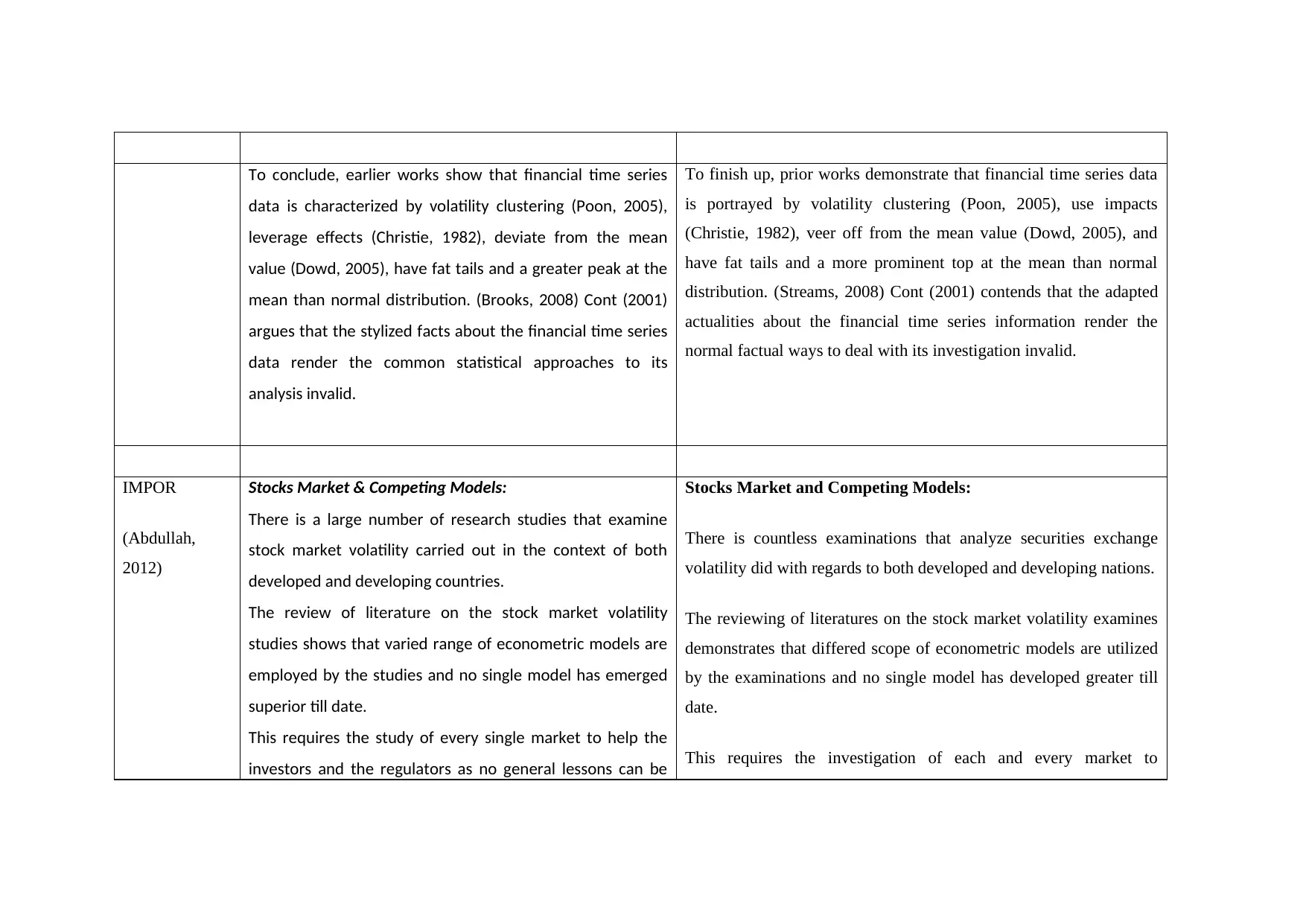
To conclude, earlier works show that financial time series
data is characterized by volatility clustering (Poon, 2005),
leverage effects (Christie, 1982), deviate from the mean
value (Dowd, 2005), have fat tails and a greater peak at the
mean than normal distribution. (Brooks, 2008) Cont (2001)
argues that the stylized facts about the financial time series
data render the common statistical approaches to its
analysis invalid.
To finish up, prior works demonstrate that financial time series data
is portrayed by volatility clustering (Poon, 2005), use impacts
(Christie, 1982), veer off from the mean value (Dowd, 2005), and
have fat tails and a more prominent top at the mean than normal
distribution. (Streams, 2008) Cont (2001) contends that the adapted
actualities about the financial time series information render the
normal factual ways to deal with its investigation invalid.
IMPOR
(Abdullah,
2012)
Stocks Market & Competing Models:
There is a large number of research studies that examine
stock market volatility carried out in the context of both
developed and developing countries.
The review of literature on the stock market volatility
studies shows that varied range of econometric models are
employed by the studies and no single model has emerged
superior till date.
This requires the study of every single market to help the
investors and the regulators as no general lessons can be
Stocks Market and Competing Models:
There is countless examinations that analyze securities exchange
volatility did with regards to both developed and developing nations.
The reviewing of literatures on the stock market volatility examines
demonstrates that differed scope of econometric models are utilized
by the examinations and no single model has developed greater till
date.
This requires the investigation of each and every market to

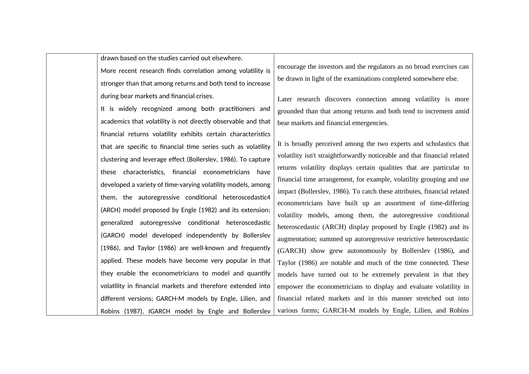
drawn based on the studies carried out elsewhere.
More recent research finds correlation among volatility is
stronger than that among returns and both tend to increase
during bear markets and financial crises.
It is widely recognized among both practitioners and
academics that volatility is not directly observable and that
financial returns volatility exhibits certain characteristics
that are specific to financial time series such as volatility
clustering and leverage effect (Bollerslev, 1986). To capture
these characteristics, financial econometricians have
developed a variety of time-varying volatility models, among
them, the autoregressive conditional heteroscedastic4
(ARCH) model proposed by Engle (1982) and its extension;
generalized autoregressive conditional heteroscedastic
(GARCH) model developed independently by Bollerslev
(1986), and Taylor (1986) are well-known and frequently
applied. These models have become very popular in that
they enable the econometricians to model and quantify
volatility in financial markets and therefore extended into
different versions; GARCH-M models by Engle, Lilien, and
Robins (1987), IGARCH model by Engle and Bollerslev
encourage the investors and the regulators as no broad exercises can
be drawn in light of the examinations completed somewhere else.
Later research discovers connection among volatility is more
grounded than that among returns and both tend to increment amid
bear markets and financial emergencies.
It is broadly perceived among the two experts and scholastics that
volatility isn't straightforwardly noticeable and that financial related
returns volatility displays certain qualities that are particular to
financial time arrangement, for example, volatility grouping and use
impact (Bollerslev, 1986). To catch these attributes, financial related
econometricians have built up an assortment of time-differing
volatility models, among them, the autoregressive conditional
heteroscedastic (ARCH) display proposed by Engle (1982) and its
augmentation; summed up autoregressive restrictive heteroscedastic
(GARCH) show grew autonomously by Bollerslev (1986), and
Taylor (1986) are notable and much of the time connected. These
models have turned out to be extremely prevalent in that they
empower the econometricians to display and evaluate volatility in
financial related markets and in this manner stretched out into
various forms; GARCH-M models by Engle, Lilien, and Robins

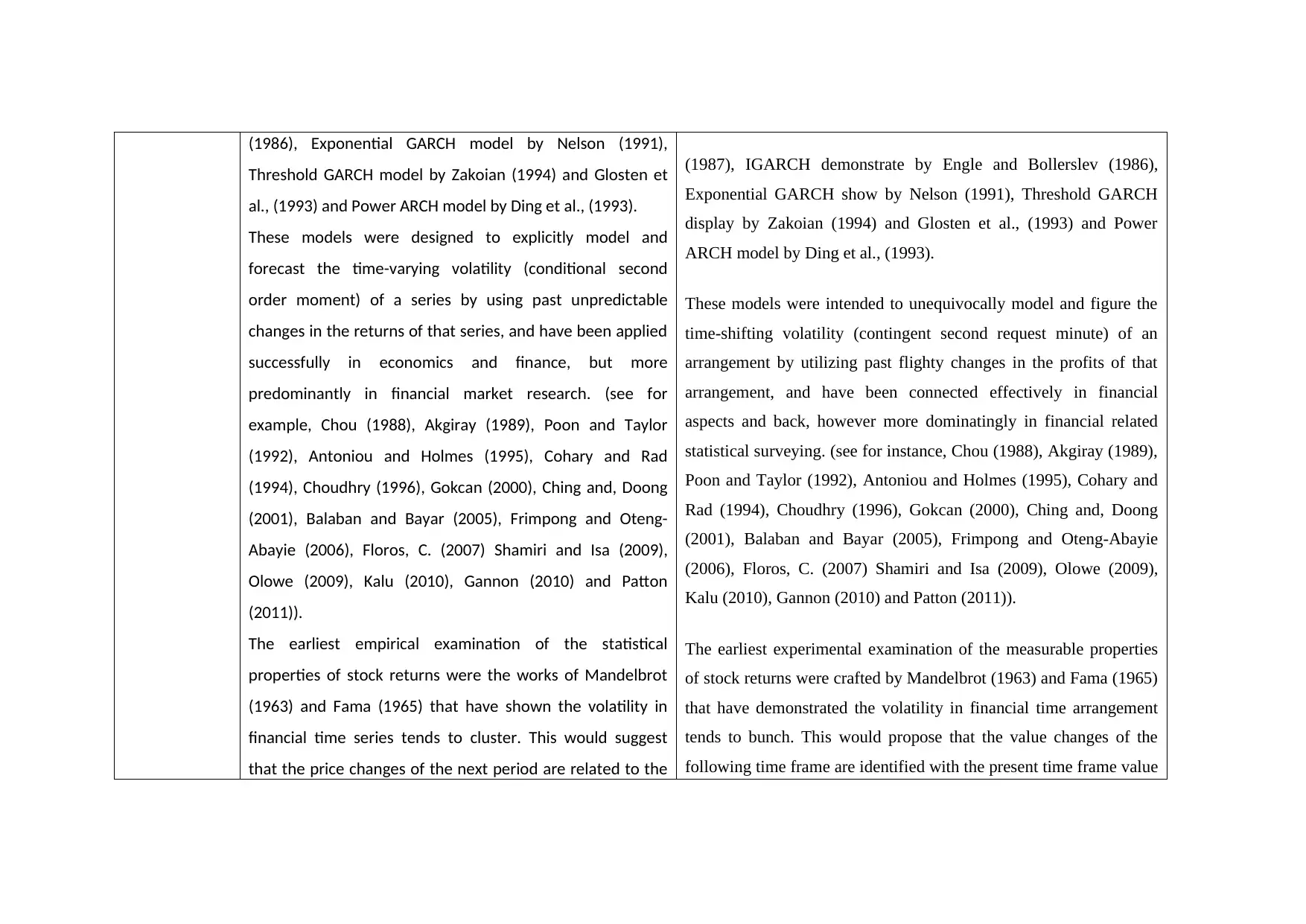
(1986), Exponential GARCH model by Nelson (1991),
Threshold GARCH model by Zakoian (1994) and Glosten et
al., (1993) and Power ARCH model by Ding et al., (1993).
These models were designed to explicitly model and
forecast the time-varying volatility (conditional second
order moment) of a series by using past unpredictable
changes in the returns of that series, and have been applied
successfully in economics and finance, but more
predominantly in financial market research. (see for
example, Chou (1988), Akgiray (1989), Poon and Taylor
(1992), Antoniou and Holmes (1995), Cohary and Rad
(1994), Choudhry (1996), Gokcan (2000), Ching and, Doong
(2001), Balaban and Bayar (2005), Frimpong and Oteng-
Abayie (2006), Floros, C. (2007) Shamiri and Isa (2009),
Olowe (2009), Kalu (2010), Gannon (2010) and Patton
(2011)).
The earliest empirical examination of the statistical
properties of stock returns were the works of Mandelbrot
(1963) and Fama (1965) that have shown the volatility in
financial time series tends to cluster. This would suggest
that the price changes of the next period are related to the
(1987), IGARCH demonstrate by Engle and Bollerslev (1986),
Exponential GARCH show by Nelson (1991), Threshold GARCH
display by Zakoian (1994) and Glosten et al., (1993) and Power
ARCH model by Ding et al., (1993).
These models were intended to unequivocally model and figure the
time-shifting volatility (contingent second request minute) of an
arrangement by utilizing past flighty changes in the profits of that
arrangement, and have been connected effectively in financial
aspects and back, however more dominatingly in financial related
statistical surveying. (see for instance, Chou (1988), Akgiray (1989),
Poon and Taylor (1992), Antoniou and Holmes (1995), Cohary and
Rad (1994), Choudhry (1996), Gokcan (2000), Ching and, Doong
(2001), Balaban and Bayar (2005), Frimpong and Oteng-Abayie
(2006), Floros, C. (2007) Shamiri and Isa (2009), Olowe (2009),
Kalu (2010), Gannon (2010) and Patton (2011)).
The earliest experimental examination of the measurable properties
of stock returns were crafted by Mandelbrot (1963) and Fama (1965)
that have demonstrated the volatility in financial time arrangement
tends to bunch. This would propose that the value changes of the
following time frame are identified with the present time frame value

current period price changes and, therefore, ensure a
predictable component of stock prices. On the same track,
Akgiray (1989) employed different ARCH and GARCH
specifications to investigate not only the time series
properties of the stock returns but also to present evidence
on the forecasting ability of ARCH and GARCH models
against some other models like EWMA (exponentially
weighted moving average) and the historic simple average
method. The empirical results revealed that GARCH model
was the best in describing and forecasting stock market
volatility. Poon and Granger (2003) provided comprehensive
review on volatility forecasting. They examined the
methodologies and empirical findings of 93 research papers
and provided synaptic view of the volatility literature on
forecasting. They found that ARCH and GARCH classes of
time series models are very useful in measuring and
forecasting volatility.
changes and, consequently, guarantee an anticipated part of stock
costs. On a similar track, Akgiray (1989) utilized diverse ARCH and
GARCH details to research not just the time arrangement properties
of the stock returns yet additionally to show confirm on the guaging
capacity of ARCH and GARCH models against some different
models like EWMA (exponentially weighted moving normal) and
the memorable straightforward normal strategy. The observational
outcomes uncovered that GARCH demonstrate was the best in
depicting and guaging securities exchange volatility. Poon and
Granger (2003) if complete survey on volatility anticipating. They
analyzed the techniques and experimental discoveries of 93 examine
papers and gave synaptic perspective of the volatility writing on
anticipating. They found that ARCH and GARCH classes of time
arrangement models are exceptionally valuable in estimating and
determining volatility.
Saudi stocks
volatility,
(Kalyanaraman
, 2014)
Overview of the KSA Stocks Market:
The Saudi stock exchange (SSE) existence dates back to
1970s when it used to operate informally. In 1984, a
Ministerial Committee comprising Ministry of Finance,
Review of the KSA Stocks Market:
The Saudi stock trade (SSE) presence goes back to 1970s when it
used to work casually. In 1984, a Ministerial Committee involving

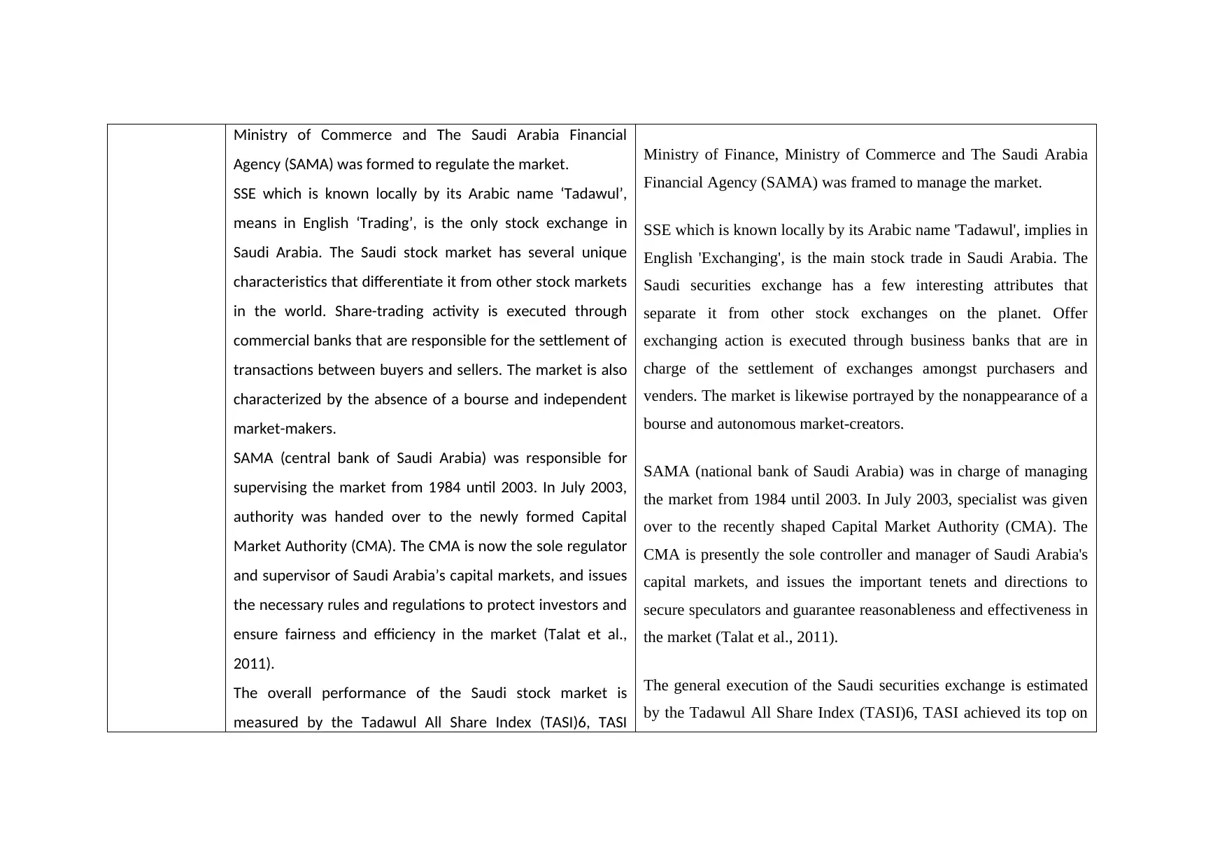
Ministry of Commerce and The Saudi Arabia Financial
Agency (SAMA) was formed to regulate the market.
SSE which is known locally by its Arabic name ‘Tadawul’,
means in English ‘Trading’, is the only stock exchange in
Saudi Arabia. The Saudi stock market has several unique
characteristics that differentiate it from other stock markets
in the world. Share-trading activity is executed through
commercial banks that are responsible for the settlement of
transactions between buyers and sellers. The market is also
characterized by the absence of a bourse and independent
market-makers.
SAMA (central bank of Saudi Arabia) was responsible for
supervising the market from 1984 until 2003. In July 2003,
authority was handed over to the newly formed Capital
Market Authority (CMA). The CMA is now the sole regulator
and supervisor of Saudi Arabia’s capital markets, and issues
the necessary rules and regulations to protect investors and
ensure fairness and efficiency in the market (Talat et al.,
2011).
The overall performance of the Saudi stock market is
measured by the Tadawul All Share Index (TASI)6, TASI
Ministry of Finance, Ministry of Commerce and The Saudi Arabia
Financial Agency (SAMA) was framed to manage the market.
SSE which is known locally by its Arabic name 'Tadawul', implies in
English 'Exchanging', is the main stock trade in Saudi Arabia. The
Saudi securities exchange has a few interesting attributes that
separate it from other stock exchanges on the planet. Offer
exchanging action is executed through business banks that are in
charge of the settlement of exchanges amongst purchasers and
venders. The market is likewise portrayed by the nonappearance of a
bourse and autonomous market-creators.
SAMA (national bank of Saudi Arabia) was in charge of managing
the market from 1984 until 2003. In July 2003, specialist was given
over to the recently shaped Capital Market Authority (CMA). The
CMA is presently the sole controller and manager of Saudi Arabia's
capital markets, and issues the important tenets and directions to
secure speculators and guarantee reasonableness and effectiveness in
the market (Talat et al., 2011).
The general execution of the Saudi securities exchange is estimated
by the Tadawul All Share Index (TASI)6, TASI achieved its top on

reached its peak on 25th of February 2006, when it closed at
20,635. It was severely affected by the 2008 global crisis,
like all the stock markets all over the world, and saw below
4000.
25th of February 2006, when it shut down at 20,635. It was
extremely influenced by the 2008 worldwide emergency, similar to
all the securities exchanges everywhere throughout the world, and
saw beneath 4000.
CMA-Crash
(2017)
Crash:
On February 25, 2006, the market had closed at its historic
high of 20,634.86. The collapse began on the following day.
By the end of 2006, the stock market’s main index, the TASI,
had lost approximately 65% of its value, and market
capitalization had fallen by half, to $326.9 billion.1
Although the intervening 11 years had not been entirely
smooth—the global financial crisis of 2008 had caused the
stock market to plummet even more than it had in 2006
The Saudi Stock Exchange (Tadawul) was established in
1985 under the supervision of the Saudi Arabian Financial
Agency (SAMA), supplanting the informal broker-based
system that had been in place since the first half of the 20th
Century. The government’s decision to establish an
Crash:
On February 25, 2006, the market had shut at its notable high of
20,634.86. The crumple started on the next day. Before the finish of
2006, the share trading system's fundamental file, the TASI, had lost
roughly 65% of its esteem, and market capitalization had fallen
considerably, to $326.9 billion.1
In spite of the fact that the mediating 11 years had not been
altogether smooth—the worldwide financial emergency of 2008 had
made the share trading system fall much more than it had in 2006
The Saudi Stock Exchange (Tadawul) was built up in 1985 under the
supervision of the Saudi Arabian Financial Agency (SAMA),
supplanting the casual specialist based framework that had been set
up since the main portion of the twentieth Century. The
administration's choice to set up a trade came in light of quick

exchange came in response to rapid growth in the number
of Saudi Arabian joint stock companies, which had
proliferated during the 1970s as the kingdom’s economy
matured. The Tadawul All Share Index (TASI), which was
assigned a base value of 1,000 in 1985, was constructed to
track the performance of all companies listed on the
exchange.3
During the early 2000s, the TASI began a steady ascent. By
year-end 2003, the TASI closed at 4,437.6, up from 2,518.1
at the end of 2002. The index rose in value by 84% in 2004
and 103.7% in 2005, closing at the end of that year at
16,712.64. The Tadawul’s market capitalization exhibited
similar growth, soaring from $68 billion in 2000 to $646
billion by year-end 2005.
Several dynamics appeared to be at play. Liquidity
throughout the region had risen. Part of this was due to
concerns after the 9/11 attacks in the United States, as
wealthy Arabs repatriated their investments from western
markets and sought to invest domestically. In addition, oil
prices had doubled between 2000 and 2005, accompanied
by global demand, and, thus, revenues from oil exports.
development in the quantity of Saudi Arabian business entities,
which had multiplied amid the 1970s as the kingdom's economy
developed. The Tadawul All Share Index (TASI), which was doled
out a base estimation of 1,000 out of 1985, was developed to track
the execution of all organizations recorded on the exchange.3
Amid the mid 2000s, the TASI started a consistent climb. By year-
end 2003, the TASI shut down at 4,437.6, up from 2,518.1 toward
the finish of 2002. The list ascended in an incentive by 84% of every
2004 and 103.7% out of 2005, shutting toward the finish of that year
at 16,712.64. The Tadawul's market capitalization displayed
comparable development, taking off from $68 billion out of 2000 to
$646 billion by year-end 2005.
A few elements seemed, by all accounts, to be at play. Liquidity all
through the area had risen. Some portion of this was because of
worries after the 9/11 assaults in the United States, as rich Arabs
repatriated their speculations from western markets and looked to
contribute locally. What's more, oil costs had multiplied somewhere
in the range of 2000 and 2005, joined by worldwide request, and,
along these lines, incomes from oil trades. Thusly, Saudi Arabia's
legislature expanded its spending on foundation, resigned obligation,

Consequently, Saudi Arabia’s government increased its
spending on infrastructure, retired debt, and invested in its
energy production systems (Al-Rodhan, 2005).
The sudden influx of retail traders posed several challenges.
They were generally unfamiliar with stock market
investment—until the early 2000s, the primary investment
assets in Saudi were real estate and gold. In addition, the
market had few large institutional investors, and practically
no international institutions to provide long-term
perspectives and dampen volatility.
Structurally, the market in Saudi was ripe for a boom and a
crash. Short-selling was not allowed. Corporate reporting
guidelines were not widely followed nor enforced. There
was very little equity research,17 and even had there been,
retail investors had little training in interpreting financial
information, and the internet offered a ready source of
uncertain information.
Reform:
In addition to set up Tadawul, the CMA had improved
disclosure rules and, in 2007, started issuing fines to
and put resources into its vitality generation frameworks (Al-
Rodhan, 2005).
The sudden deluge of retail merchants represented a few difficulties.
They were for the most part new to securities exchange speculation
—until the mid 2000s, the essential venture resources in Saudi were
land and gold. What's more, the market had couple of substantial
institutional financial specialists, and for all intents and purposes no
global organizations to give long haul points of view and hose
volatility.
Fundamentally, the market in Saudi was ready for a blast and a
crash. Short-offering was not permitted. Corporate announcing rules
were not generally taken after nor implemented. There was almost
no value research,17 and even had there been, retail speculators had
small preparing in deciphering financial related data, and the web
offered a prepared wellspring of dubious data.
Change:
Notwithstanding set up Tadawul, the CMA had enhanced revelation
rules and, in 2007, began issuing fines to organizations that did not

companies that did not provide their reports on time.
Foreign investment groups could now trade in the market, a
change the CMA hoped would provide additional stability.
Among reforms CMA enacted as steps to increase disclosure
and transparency and enforce regulations, encouraging
large private companies to list and increase the number of
companies in the public markets and improve stability.
The CMA’s recent decision to open a new secondary board,
the “Parallel Market,” that was specifically designed to ease
the regulatory burden of going public for small-and
medium-sized entities (SMEs), represented an important
step in the right direction. The more relaxed regulations
included just one year of audited financials. Sophisticated
investors would need to research the companies on the
Parallel Market. With the recently adopted IPO pricing
approach of book building, the issues around under-pricing
could be addressed.
give their reports on time. Outside speculation gatherings could now
exchange the market, a change the CMA trusted would give extra
security.
Among changes CMA authorized as ventures to expand revelation
and straightforwardness and implement directions, urging huge
privately owned businesses to rundown and increment the quantity
of organizations in the general population showcases and enhance
security.
The CMA's ongoing choice to open another optional board, the
"Parallel Market," that was particularly intended to facilitate the
administrative weight of opening up to the world for little and
medium-sized substances (SMEs), spoke to an essential positive
development. The more casual directions included only one year of
inspected financials. Complex speculators would need to look into
the organizations on the Parallel Market. With the as of late
embraced IPO evaluating methodology of book constructing, the
issues around under-estimating could be tended to.