Water and Sewer for Queensland

This report presents the design for an upgrade of a water supply system and a sanitary sewer for an area in Queensland. It covers population projection, the Hardy-Cross method, and more. The report is a valuable resource for students studying water supply and sewer design.

Water and Sewer for Queensland 1
WATER AND SEWER FOR QUEENSLAND
By [Name]
Course
Professor’s Name
Institution
Location of Institution
Date

Water and Sewer for Queensland 2
Water Supply Pipeline and Sanitary Sewer Design
Introduction
The main task in this report was to design for an upgrade of a water supply system and a sanitary sewer for the same area of a
town in Queensland. The designs were done and the report is presented below.
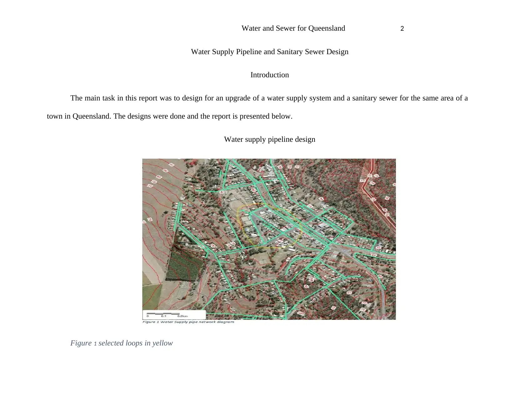
Water supply pipeline design
Figure 1 selected loops in yellow

Water and Sewer for Queensland 3
Population Projection
The loops to be designed were selected and have been marked from the overall area. We counted the houses physically for the
area demarcated and they were found to be approximately 57 houses. With the approximate on three people per house and a growth
rate of 1.4% according to the Australian Bureau of Statistics (Australian Bureau of Statistics, 2018), the population was approximated
at 232 by the year 2040 which was taken as the ultimate design year. With the daily demand of 171l/c/d according to (Anon., 2017)
the domestic water demand was found to be 39672l/d.
The populations were as follows:
Current population Year 2018 171
Base year population 2020 176
Future design Year 2030 202
Ultimate design Year 2040 232
On top of the domestic water demand, an overall percentage of 37% was added to cater for unaccounted for water,
institutional, commercial and fire demands for the region according to the analysis done for the area. Adding this demand on the
domestic demand, the total demand for the area was found to be 54350.6 l/d, which translates to 0.64l/s.

Water and Sewer for Queensland 4
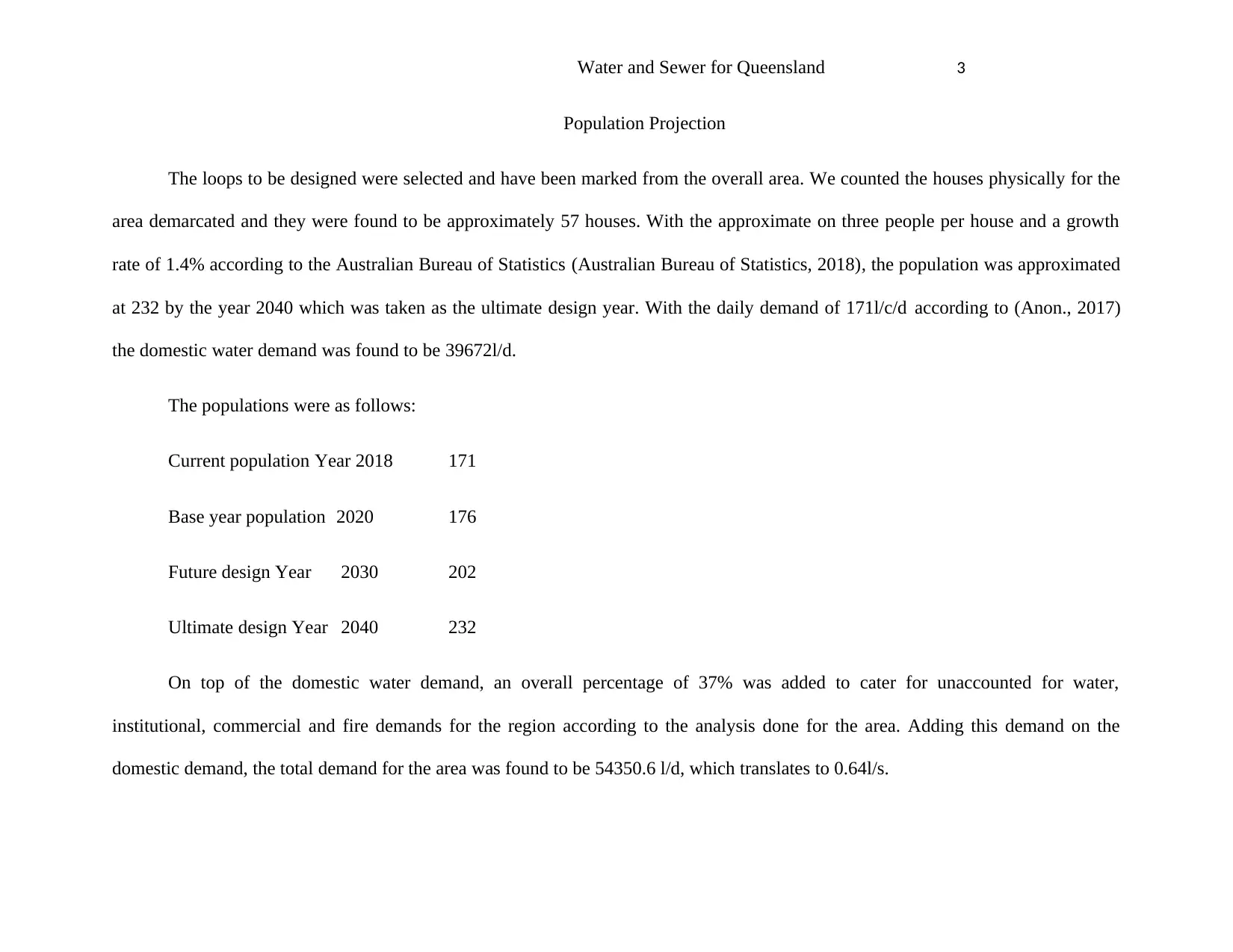
Below is the table showing how the population was projected by the use of linear population projection formulae.
Year 2018 2020 2030 2040
Population 171 176 202 232
Domestic water demand{l/d} 29241 30096 34542 39672
Unaccounted for water {l/d} 4386.15 4514.4 5181.3 5950.8
Institutional demand{l/d} 5848.2 6019.2 6908.4 7934.4
Fire demand{l/d} 584.82 601.92 690.84 793.44
Total demand{l/d} 40060.2 41231.52 47322.54 54350.6
Table 1 Calculation of Water Demand.
The total demand was distributed equally to all the junctions for the loop that was selected.
The analysis was done using the hardy cross method to determine the flows, velocities, and head-losses for the system that was
designed. This method achieves the solution by several iterations to find the correct flows.
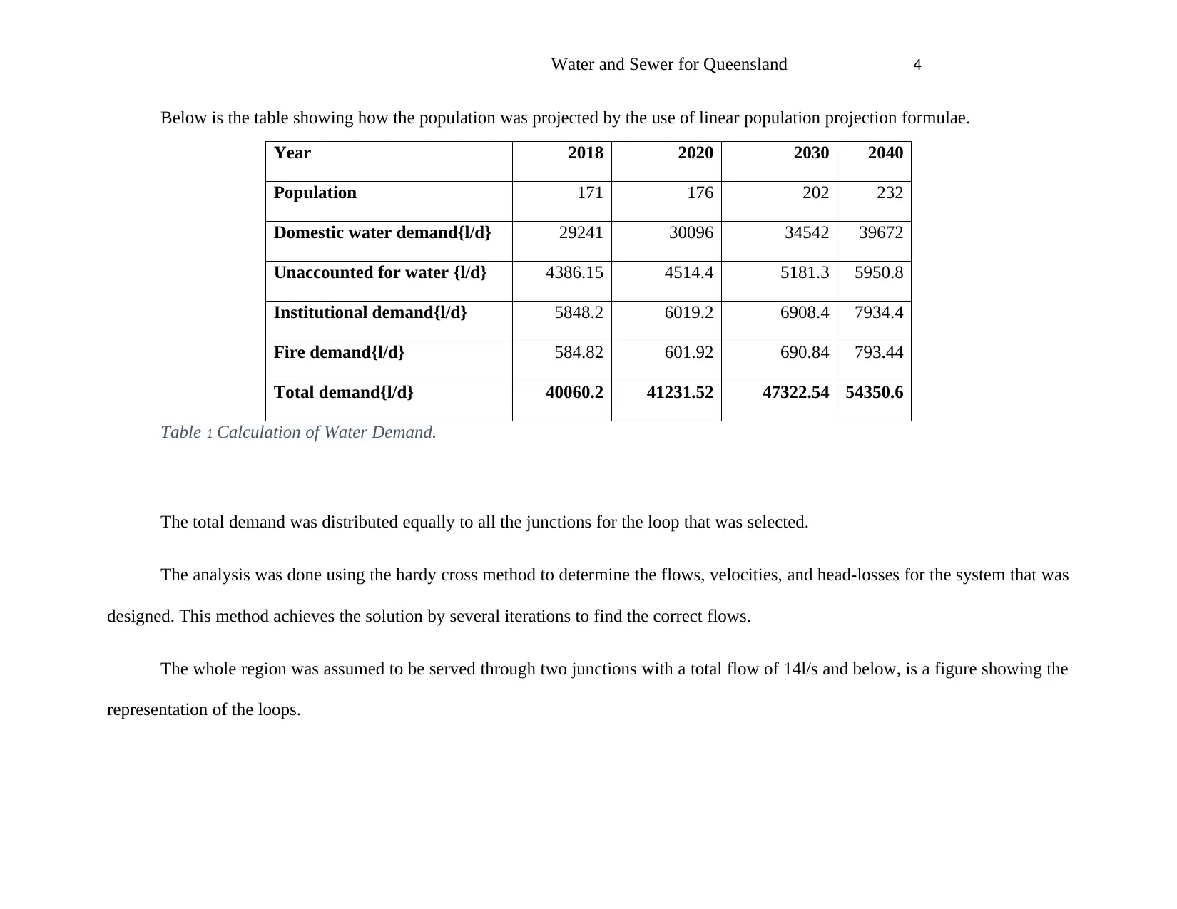
The whole region was assumed to be served through two junctions with a total flow of 14l/s and below, is a figure showing the
representation of the loops.

Water and Sewer for Queensland 5
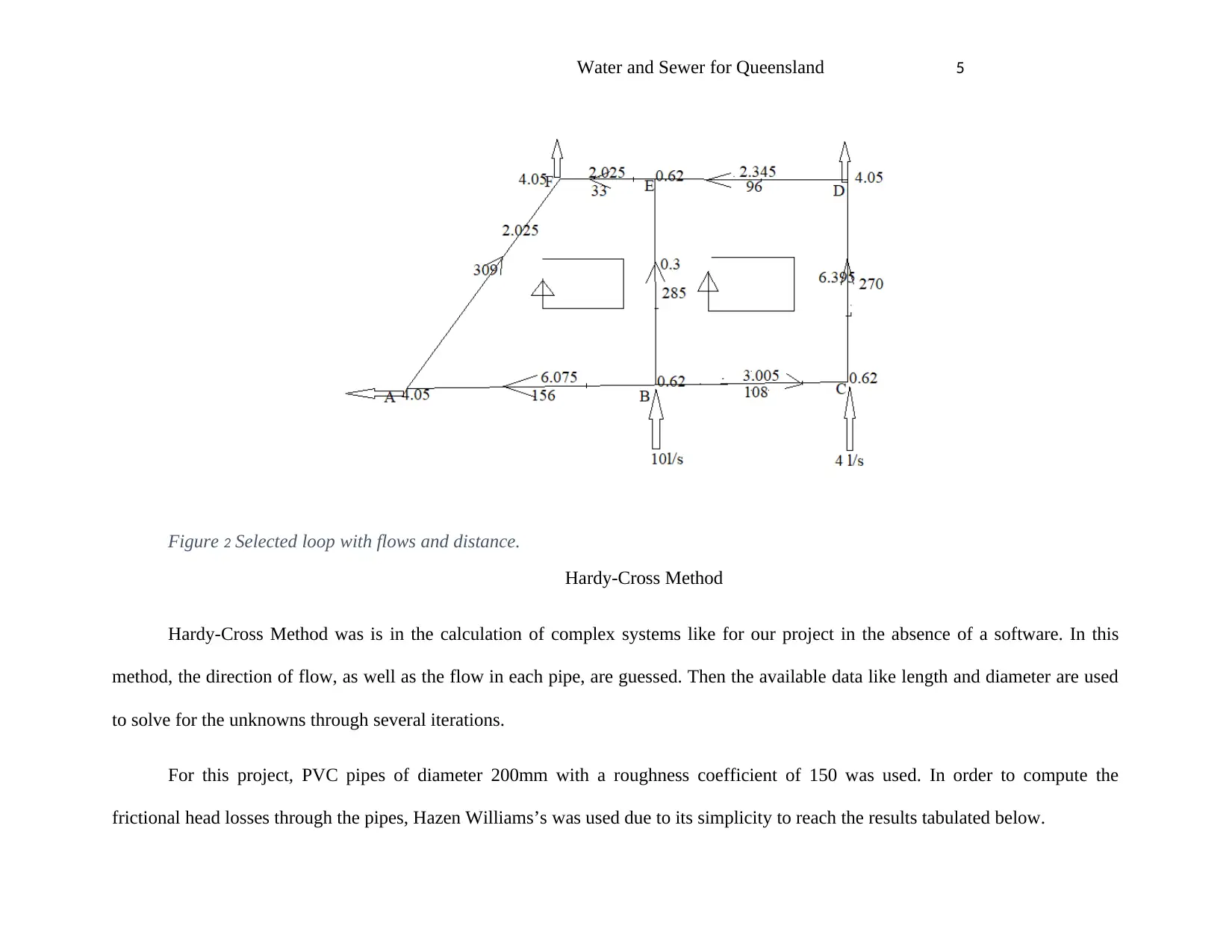
Figure 2 Selected loop with flows and distance.
Hardy-Cross Method
Hardy-Cross Method was is in the calculation of complex systems like for our project in the absence of a software. In this
method, the direction of flow, as well as the flow in each pipe, are guessed. Then the available data like length and diameter are used
to solve for the unknowns through several iterations.
For this project, PVC pipes of diameter 200mm with a roughness coefficient of 150 was used. In order to compute the
frictional head losses through the pipes, Hazen Williams’s was used due to its simplicity to reach the results tabulated below.

Water and Sewer for Queensland 6
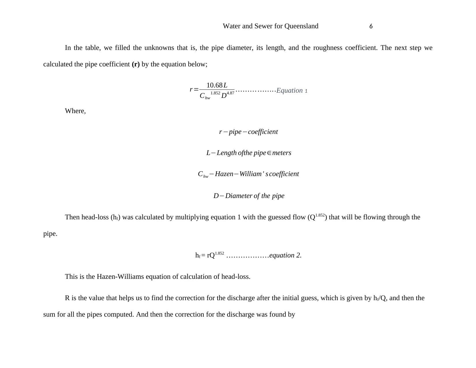
In the table, we filled the unknowns that is, the pipe diameter, its length, and the roughness coefficient. The next step we
calculated the pipe coefficient (r) by the equation below;
r = 10.68 L
Chw
1.852 D4.87 … … … … …. .Equation 1
Where,
r −pipe−coefficient
L−Length ofthe pipe∈meters
Chw−Hazen−William' s coefficient
D−Diameter of the pipe
Then head-loss (hf) was calculated by multiplying equation 1 with the guessed flow (Q1.852) that will be flowing through the
pipe.
hf = rQ1.852 ………………equation 2.
This is the Hazen-Williams equation of calculation of head-loss.
R is the value that helps us to find the correction for the discharge after the initial guess, which is given by hf/Q, and then the
sum for all the pipes computed. And then the correction for the discharge was found by

Water and Sewer for Queensland 7
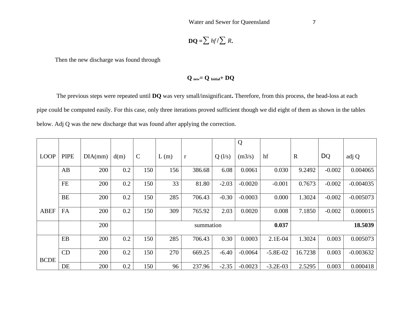
DQ =∑ hf /∑ R.
Then the new discharge was found through
Q new= Q Initial+ DQ
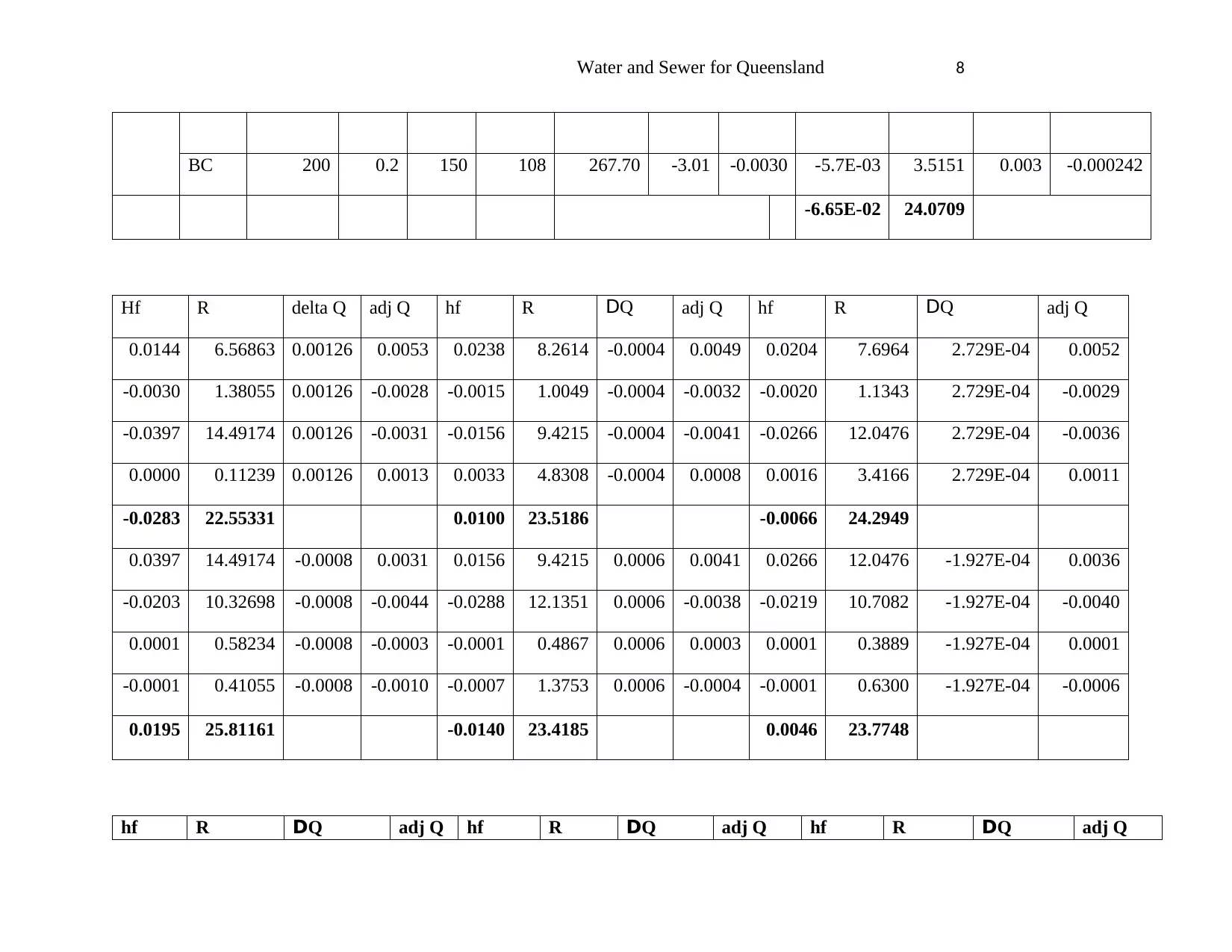
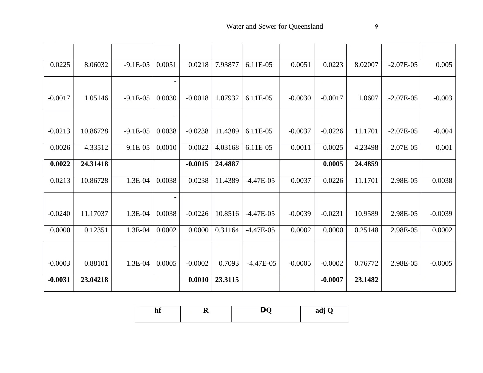
The previous steps were repeated until DQ was very small/insignificant. Therefore, from this process, the head-loss at each
pipe could be computed easily. For this case, only three iterations proved sufficient though we did eight of them as shown in the tables
below. Adj Q was the new discharge that was found after applying the correction.
LOOP PIPE DIA(mm) d(m) C L (m) r Q (l/s)
Q
(m3/s) hf R DQ adj Q
ABEF
AB 200 0.2 150 156 386.68 6.08 0.0061 0.030 9.2492 -0.002 0.004065
FE 200 0.2 150 33 81.80 -2.03 -0.0020 -0.001 0.7673 -0.002 -0.004035
BE 200 0.2 150 285 706.43 -0.30 -0.0003 0.000 1.3024 -0.002 -0.005073
FA 200 0.2 150 309 765.92 2.03 0.0020 0.008 7.1850 -0.002 0.000015
200 summation 0.037 18.5039
BCDE
EB 200 0.2 150 285 706.43 0.30 0.0003 2.1E-04 1.3024 0.003 0.005073
CD 200 0.2 150 270 669.25 -6.40 -0.0064 -5.8E-02 16.7238 0.003 -0.003632
DE 200 0.2 150 96 237.96 -2.35 -0.0023 -3.2E-03 2.5295 0.003 0.000418

Water and Sewer for Queensland 8
BC 200 0.2 150 108 267.70 -3.01 -0.0030 -5.7E-03 3.5151 0.003 -0.000242
-6.65E-02 24.0709
Hf R delta Q adj Q hf R DQ adj Q hf R DQ adj Q
0.0144 6.56863 0.00126 0.0053 0.0238 8.2614 -0.0004 0.0049 0.0204 7.6964 2.729E-04 0.0052
-0.0030 1.38055 0.00126 -0.0028 -0.0015 1.0049 -0.0004 -0.0032 -0.0020 1.1343 2.729E-04 -0.0029
-0.0397 14.49174 0.00126 -0.0031 -0.0156 9.4215 -0.0004 -0.0041 -0.0266 12.0476 2.729E-04 -0.0036
0.0000 0.11239 0.00126 0.0013 0.0033 4.8308 -0.0004 0.0008 0.0016 3.4166 2.729E-04 0.0011
-0.0283 22.55331 0.0100 23.5186 -0.0066 24.2949
0.0397 14.49174 -0.0008 0.0031 0.0156 9.4215 0.0006 0.0041 0.0266 12.0476 -1.927E-04 0.0036
-0.0203 10.32698 -0.0008 -0.0044 -0.0288 12.1351 0.0006 -0.0038 -0.0219 10.7082 -1.927E-04 -0.0040
0.0001 0.58234 -0.0008 -0.0003 -0.0001 0.4867 0.0006 0.0003 0.0001 0.3889 -1.927E-04 0.0001
-0.0001 0.41055 -0.0008 -0.0010 -0.0007 1.3753 0.0006 -0.0004 -0.0001 0.6300 -1.927E-04 -0.0006
0.0195 25.81161 -0.0140 23.4185 0.0046 23.7748
hf R DQ adj Q hf R DQ adj Q hf R DQ adj Q

Water and Sewer for Queensland 9
0.0225 8.06032 -9.1E-05 0.0051 0.0218 7.93877 6.11E-05 0.0051 0.0223 8.02007 -2.07E-05 0.005
-0.0017 1.05146 -9.1E-05
-
0.0030 -0.0018 1.07932 6.11E-05 -0.0030 -0.0017 1.0607 -2.07E-05 -0.003
-0.0213 10.86728 -9.1E-05
-
0.0038 -0.0238 11.4389 6.11E-05 -0.0037 -0.0226 11.1701 -2.07E-05 -0.004
0.0026 4.33512 -9.1E-05 0.0010 0.0022 4.03168 6.11E-05 0.0011 0.0025 4.23498 -2.07E-05 0.001
0.0022 24.31418 -0.0015 24.4887 0.0005 24.4859
0.0213 10.86728 1.3E-04 0.0038 0.0238 11.4389 -4.47E-05 0.0037 0.0226 11.1701 2.98E-05 0.0038
-0.0240 11.17037 1.3E-04
-
0.0038 -0.0226 10.8516 -4.47E-05 -0.0039 -0.0231 10.9589 2.98E-05 -0.0039
0.0000 0.12351 1.3E-04 0.0002 0.0000 0.31164 -4.47E-05 0.0002 0.0000 0.25148 2.98E-05 0.0002
-0.0003 0.88101 1.3E-04
-
0.0005 -0.0002 0.7093 -4.47E-05 -0.0005 -0.0002 0.76772 2.98E-05 -0.0005
-0.0031 23.04218 0.0010 23.3115 -0.0007 23.1482
hf R DQ adj Q

Water and Sewer for Queensland 10
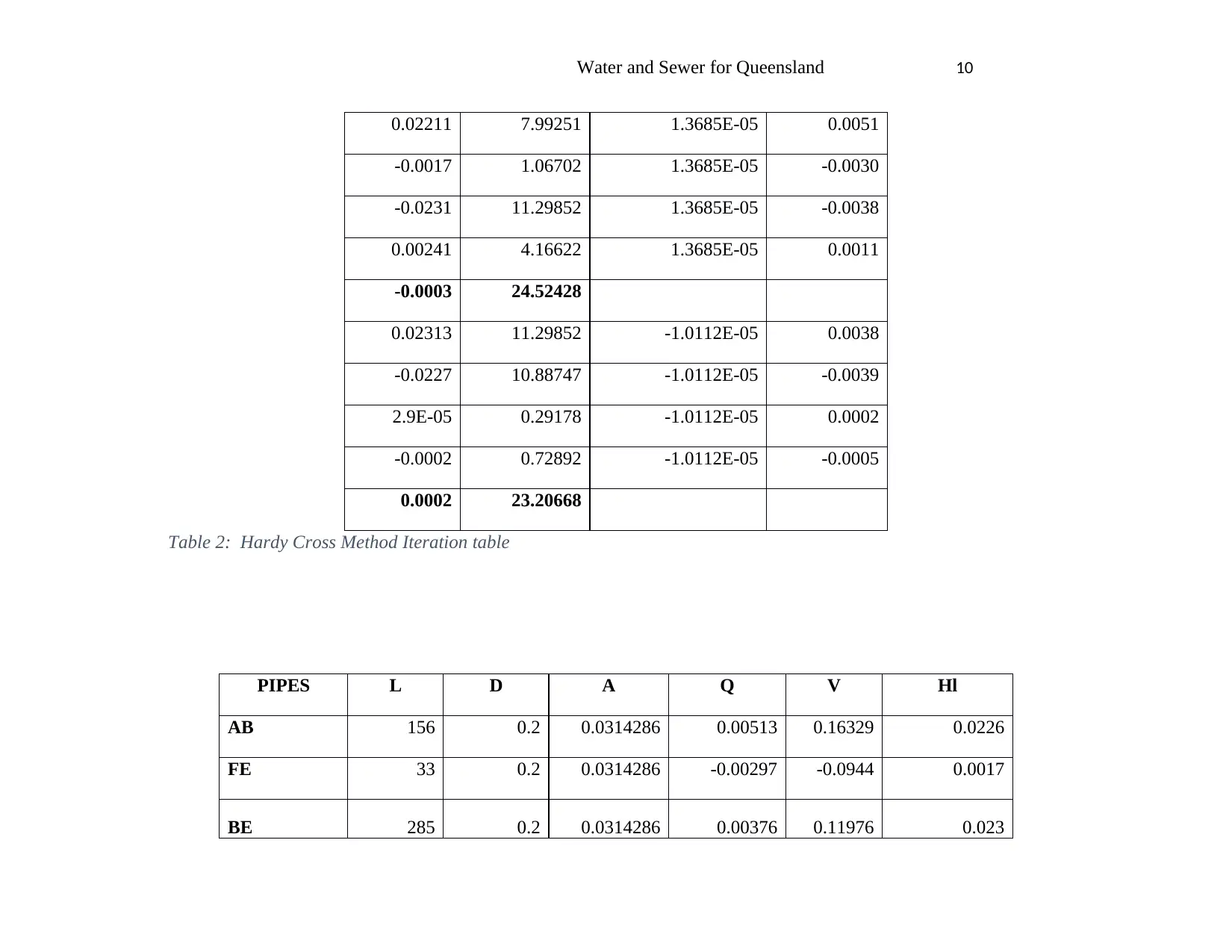
0.02211 7.99251 1.3685E-05 0.0051
-0.0017 1.06702 1.3685E-05 -0.0030
-0.0231 11.29852 1.3685E-05 -0.0038
0.00241 4.16622 1.3685E-05 0.0011
-0.0003 24.52428
0.02313 11.29852 -1.0112E-05 0.0038
-0.0227 10.88747 -1.0112E-05 -0.0039
2.9E-05 0.29178 -1.0112E-05 0.0002
-0.0002 0.72892 -1.0112E-05 -0.0005
0.0002 23.20668
Table 2: Hardy Cross Method Iteration table
PIPES L D A Q V Hl
AB 156 0.2 0.0314286 0.00513 0.16329 0.0226
FE 33 0.2 0.0314286 -0.00297 -0.0944 0.0017
BE 285 0.2 0.0314286 0.00376 0.11976 0.023

Water and Sewer for Queensland 11
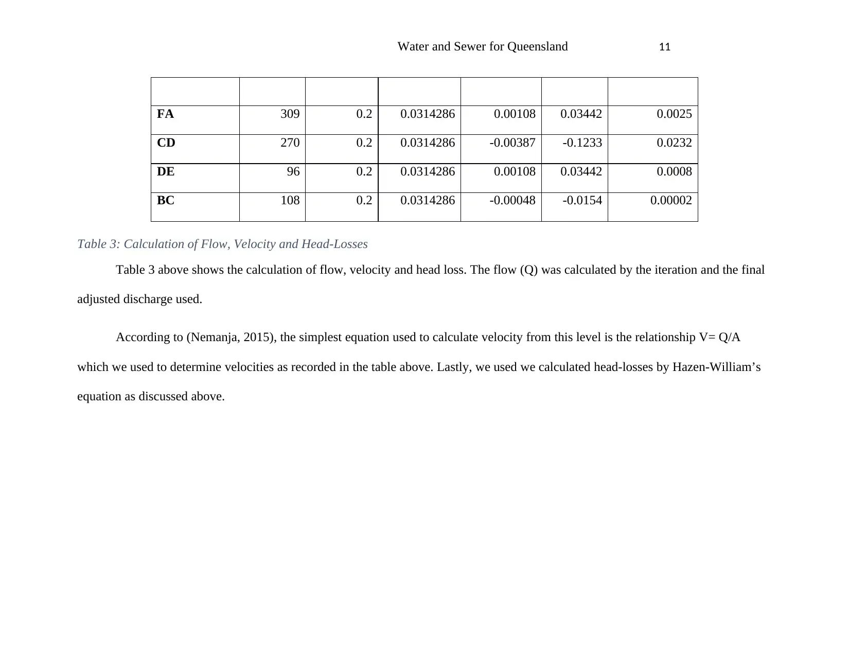
FA 309 0.2 0.0314286 0.00108 0.03442 0.0025
CD 270 0.2 0.0314286 -0.00387 -0.1233 0.0232
DE 96 0.2 0.0314286 0.00108 0.03442 0.0008
BC 108 0.2 0.0314286 -0.00048 -0.0154 0.00002
Table 3: Calculation of Flow, Velocity and Head-Losses
Table 3 above shows the calculation of flow, velocity and head loss. The flow (Q) was calculated by the iteration and the final
adjusted discharge used.
According to (Nemanja, 2015), the simplest equation used to calculate velocity from this level is the relationship V= Q/A
which we used to determine velocities as recorded in the table above. Lastly, we used we calculated head-losses by Hazen-William’s
equation as discussed above.

Water and Sewer for Queensland 12
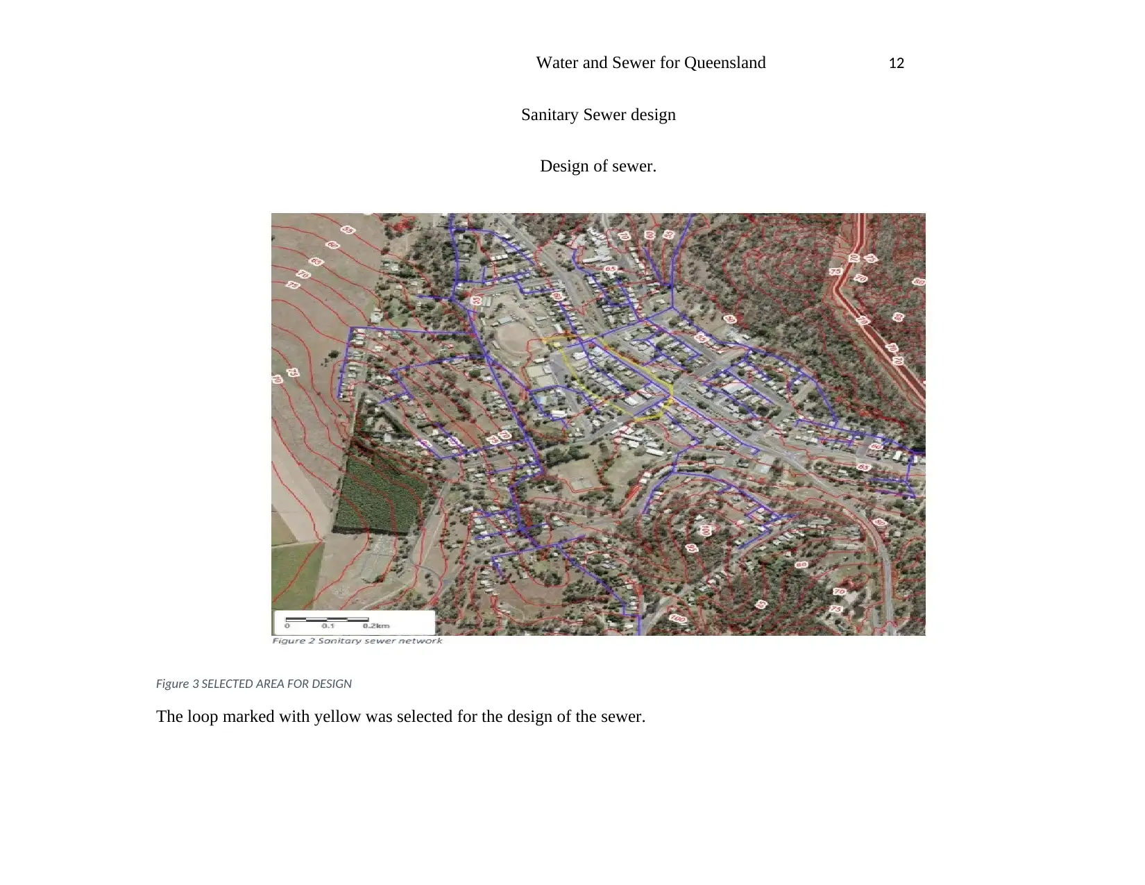
Sanitary Sewer design
Design of sewer.
Figure 3 SELECTED AREA FOR DESIGN
The loop marked with yellow was selected for the design of the sewer.

Water and Sewer for Queensland 13
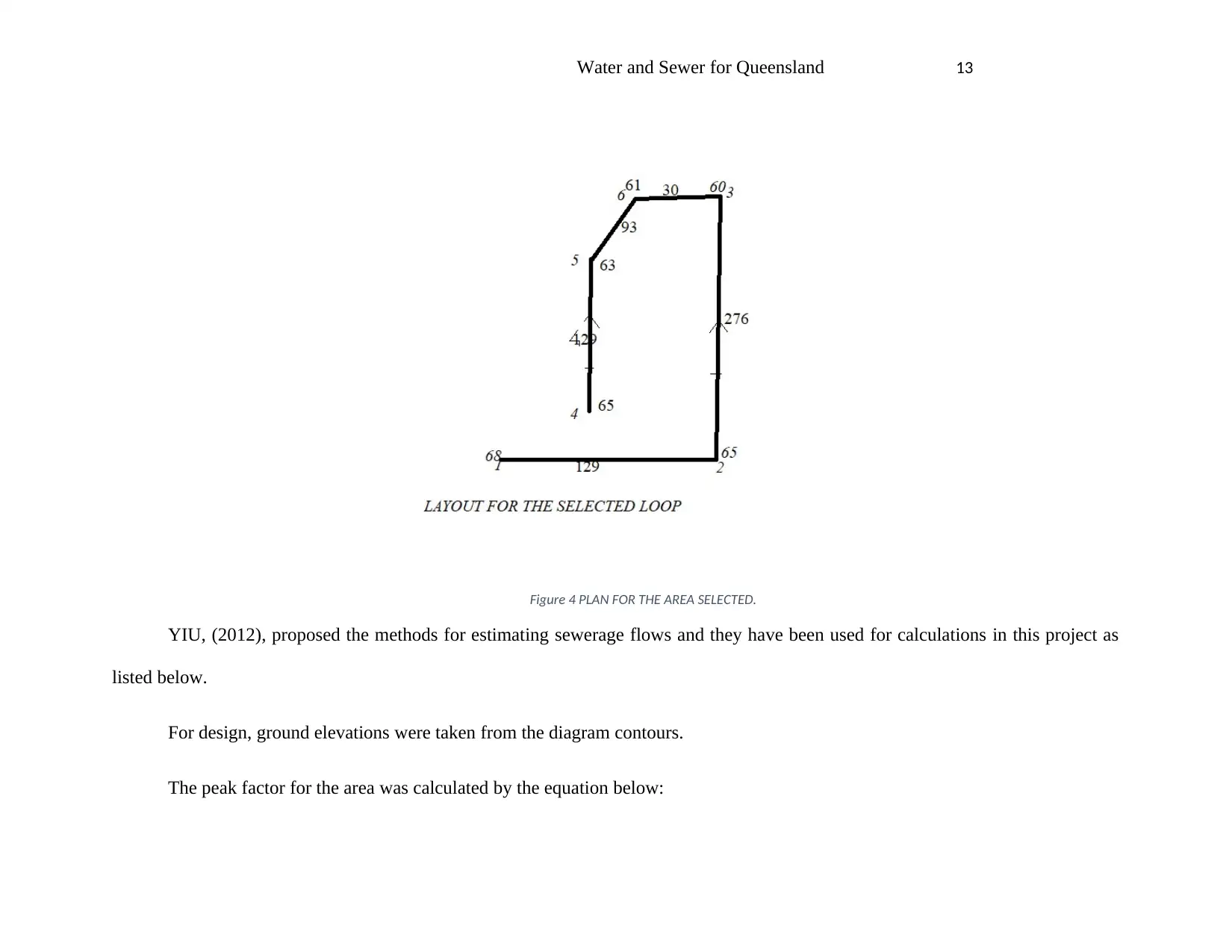
Figure 4 PLAN FOR THE AREA SELECTED.
YIU, (2012), proposed the methods for estimating sewerage flows and they have been used for calculations in this project as
listed below.
For design, ground elevations were taken from the diagram contours.
The peak factor for the area was calculated by the equation below:

Water and Sewer for Queensland 14
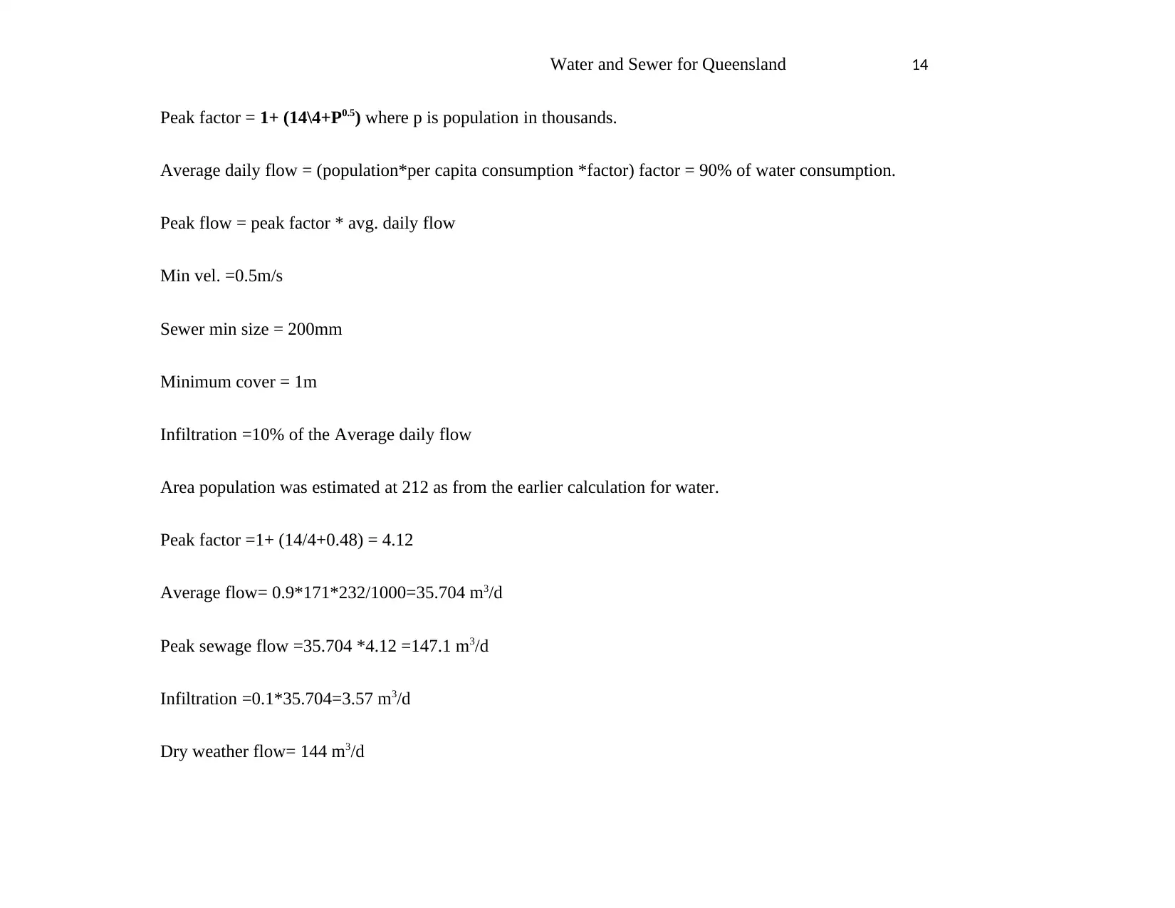
Peak factor = 1+ (14\4+P0.5) where p is population in thousands.
Average daily flow = (population*per capita consumption *factor) factor = 90% of water consumption.
Peak flow = peak factor * avg. daily flow
Min vel. =0.5m/s
Sewer min size = 200mm
Minimum cover = 1m
Infiltration =10% of the Average daily flow
Area population was estimated at 212 as from the earlier calculation for water.
Peak factor =1+ (14/4+0.48) = 4.12
Average flow= 0.9*171*232/1000=35.704 m3/d
Peak sewage flow =35.704 *4.12 =147.1 m3/d
Infiltration =0.1*35.704=3.57 m3/d
Dry weather flow= 144 m3/d

Water and Sewer for Queensland 15
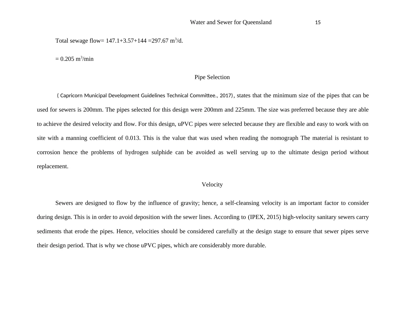
Total sewage flow= 147.1+3.57+144 =297.67 m3/d.
= 0.205 m3/min
Pipe Selection
( Capricorn Municipal Development Guidelines Technical Committee., 2017), states that the minimum size of the pipes that can be
used for sewers is 200mm. The pipes selected for this design were 200mm and 225mm. The size was preferred because they are able
to achieve the desired velocity and flow. For this design, uPVC pipes were selected because they are flexible and easy to work with on
site with a manning coefficient of 0.013. This is the value that was used when reading the nomograph The material is resistant to
corrosion hence the problems of hydrogen sulphide can be avoided as well serving up to the ultimate design period without
replacement.
Velocity
Sewers are designed to flow by the influence of gravity; hence, a self-cleansing velocity is an important factor to consider
during design. This is in order to avoid deposition with the sewer lines. According to (IPEX, 2015) high-velocity sanitary sewers carry
sediments that erode the pipes. Hence, velocities should be considered carefully at the design stage to ensure that sewer pipes serve
their design period. That is why we chose uPVC pipes, which are considerably more durable.

Water and Sewer for Queensland 16
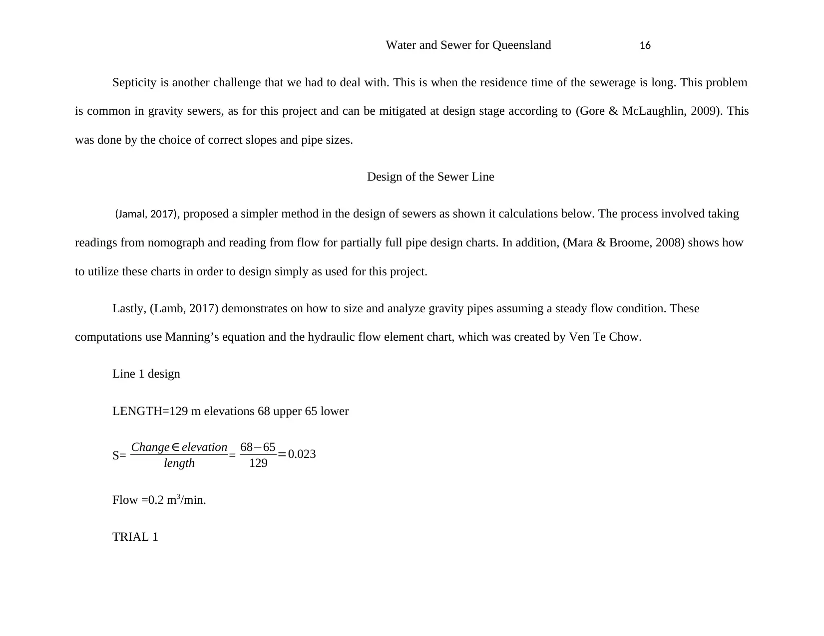
Septicity is another challenge that we had to deal with. This is when the residence time of the sewerage is long. This problem
is common in gravity sewers, as for this project and can be mitigated at design stage according to (Gore & McLaughlin, 2009). This
was done by the choice of correct slopes and pipe sizes.
Design of the Sewer Line
(Jamal, 2017), proposed a simpler method in the design of sewers as shown it calculations below. The process involved taking
readings from nomograph and reading from flow for partially full pipe design charts. In addition, (Mara & Broome, 2008) shows how
to utilize these charts in order to design simply as used for this project.
Lastly, (Lamb, 2017) demonstrates on how to size and analyze gravity pipes assuming a steady flow condition. These
computations use Manning’s equation and the hydraulic flow element chart, which was created by Ven Te Chow.
Line 1 design
LENGTH=129 m elevations 68 upper 65 lower
S= Change∈ elevation
length = 68−65
129 =0.023
Flow =0.2 m3/min.
TRIAL 1

Water and Sewer for Queensland 17
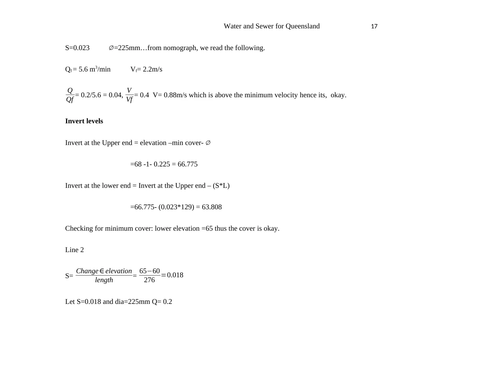
S=0.023 ∅ =225mm…from nomograph, we read the following.
Qf = 5.6 m3/min Vf= 2.2m/s
Q
Qf = 0.2/5.6 = 0.04, V
Vf = 0.4 V= 0.88m/s which is above the minimum velocity hence its, okay.
Invert levels
Invert at the Upper end = elevation –min cover- ∅
=68 -1- 0.225 = 66.775
Invert at the lower end = Invert at the Upper end – (S*L)
=66.775- (0.023*129) = 63.808
Checking for minimum cover: lower elevation =65 thus the cover is okay.
Line 2
S= Change∈ elevation
length = 65−60
276 =0.018
Let S=0.018 and dia=225mm Q= 0.2

Water and Sewer for Queensland 18
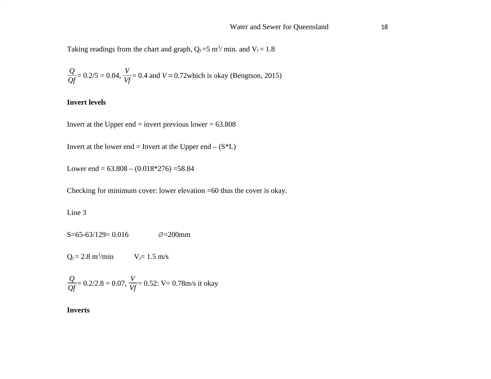
Taking readings from the chart and graph, Qf =5 m3/ min. and Vf = 1.8
Q
Qf = 0.2/5 = 0.04, V
Vf = 0.4 and V =0.72which is okay (Bengtson, 2015)
Invert levels
Invert at the Upper end = invert previous lower = 63.808
Invert at the lower end = Invert at the Upper end – (S*L)
Lower end = 63.808 – (0.018*276) =58.84
Checking for minimum cover: lower elevation =60 thus the cover is okay.
Line 3
S=65-63/129= 0.016 ∅ =200mm
Qf = 2.8 m3/min Vf= 1.5 m/s
Q
Qf = 0.2/2.8 = 0.07, V
Vf = 0.52: V= 0.78m/s it okay
Inverts

Water and Sewer for Queensland 19
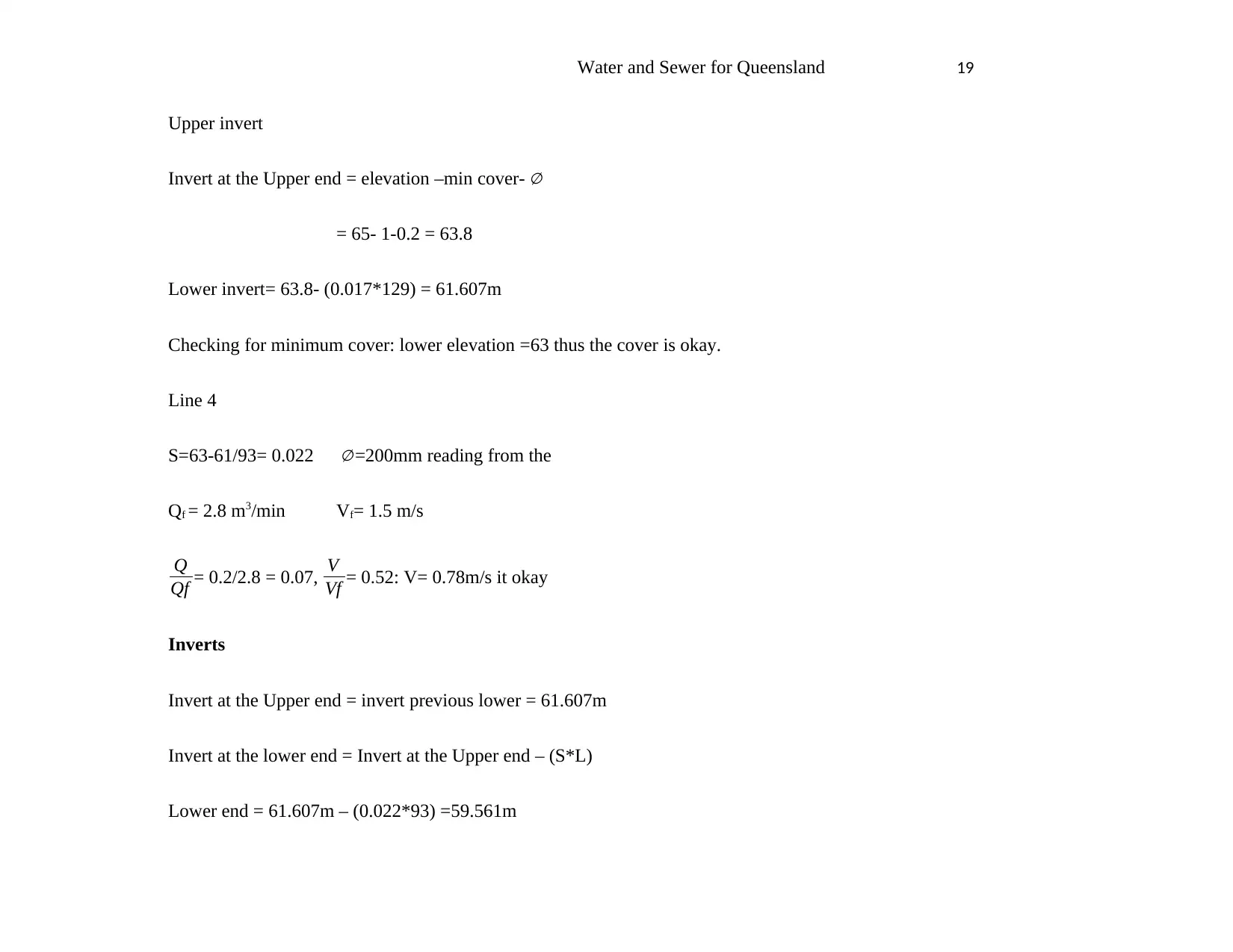
Upper invert
Invert at the Upper end = elevation –min cover- ∅
= 65- 1-0.2 = 63.8
Lower invert= 63.8- (0.017*129) = 61.607m
Checking for minimum cover: lower elevation =63 thus the cover is okay.
Line 4
S=63-61/93= 0.022 ∅ =200mm reading from the
Qf = 2.8 m3/min Vf= 1.5 m/s
Q
Qf = 0.2/2.8 = 0.07, V
Vf = 0.52: V= 0.78m/s it okay
Inverts
Invert at the Upper end = invert previous lower = 61.607m
Invert at the lower end = Invert at the Upper end – (S*L)
Lower end = 61.607m – (0.022*93) =59.561m

Water and Sewer for Queensland 20
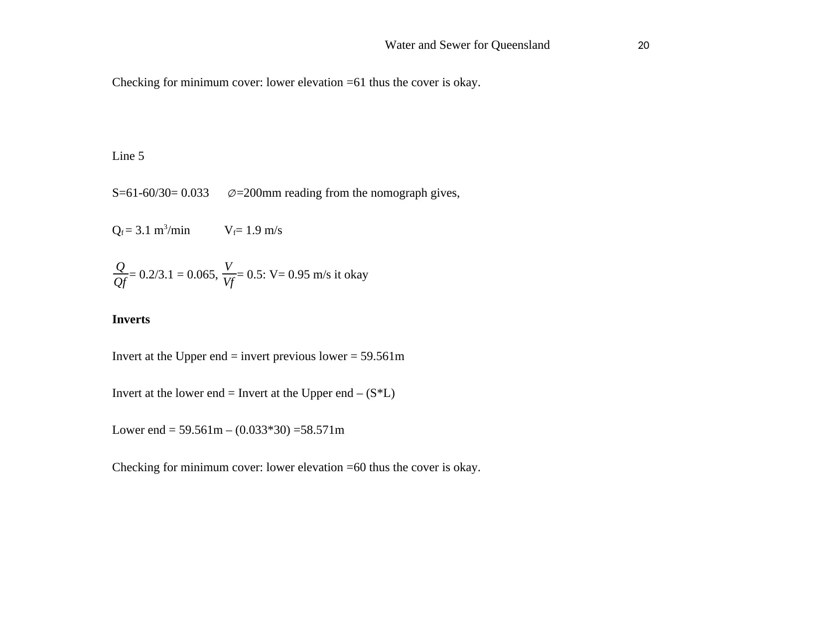
Checking for minimum cover: lower elevation =61 thus the cover is okay.
Line 5
S=61-60/30= 0.033 ∅ =200mm reading from the nomograph gives,
Qf = 3.1 m3/min Vf= 1.9 m/s
Q
Qf = 0.2/3.1 = 0.065, V
Vf = 0.5: V= 0.95 m/s it okay
Inverts
Invert at the Upper end = invert previous lower = 59.561m
Invert at the lower end = Invert at the Upper end – (S*L)
Lower end = 59.561m – (0.033*30) =58.571m
Checking for minimum cover: lower elevation =60 thus the cover is okay.

Water and Sewer for Queensland 21
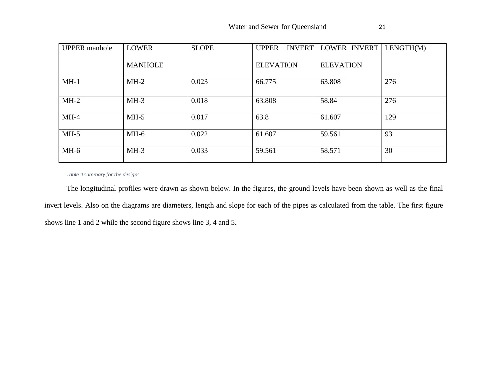
Table 4 summary for the designs
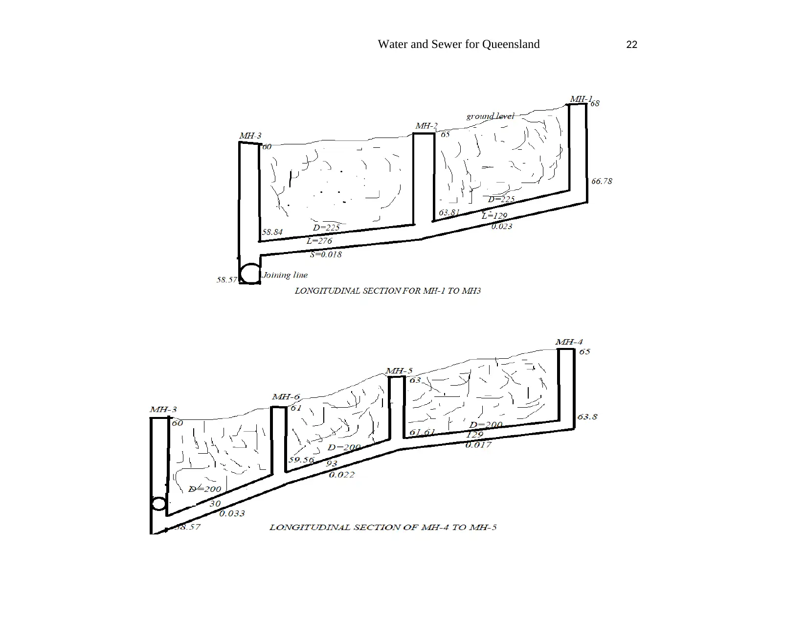
The longitudinal profiles were drawn as shown below. In the figures, the ground levels have been shown as well as the final
invert levels. Also on the diagrams are diameters, length and slope for each of the pipes as calculated from the table. The first figure
shows line 1 and 2 while the second figure shows line 3, 4 and 5.
UPPER manhole LOWER
MANHOLE
SLOPE UPPER INVERT
ELEVATION
LOWER INVERT
ELEVATION
LENGTH(M)
MH-1 MH-2 0.023 66.775 63.808 276
MH-2 MH-3 0.018 63.808 58.84 276
MH-4 MH-5 0.017 63.8 61.607 129
MH-5 MH-6 0.022 61.607 59.561 93
MH-6 MH-3 0.033 59.561 58.571 30

Water and Sewer for Queensland 22

Water and Sewer for Queensland 23
Conclusion
In the design of sewers, both the nomograph and partially full flow charts for Manning’s equation were used. These charts
were used simultaneously in order to determine flow when full (Qf) and velocities (Vf) and were used to find the flow. We only
needed to know the slope and the size of the pipe used. If the first trial failed by giving a velocity that is below the minimum, flow
could be used with a different slope.

Water and Sewer for Queensland 24
References
Capricorn Municipal Development Guidelines Technical Committee., 2017. Capricorn Municipal Development Guidelines.
[Online]
Available at: http://www.cmdg.com.au/Guidelines/GuidelinesHome.html
[Accessed 25 july 2018].
Anon., 2017. ABCDiamond Australia Australian Information. [Online]
Available at: https://abcdiamond.com.au/average-daily-residential-water-consumption-in-queensland/
[Accessed 7 8 2018].
Australian Bureau of Statistics, 2018. [Online]
Available at: http://www.abs.gov.au/AUSSTATS/abs@.nsf/Web+Pages/Population+Clock?opendocument&ref=HPKI
[Accessed July 2018].
Bengtson, H. H., 2015. Spreadsheet Use for Partially Full Pipe Flow Calculation. Greyridge Farm Court: CED
Engineering.com.
DRAINAGE SERVICES DEPARTMENT, 2013. Key Planning Issues and Gravity Collection System. 3rd ed. Hong Kong:
Government of Hong Kong.
Gore, M. & McLaughlin, C., 2009. Septicity Occurrence and Mitigation Within Wastewater Transfer Systems. Tamworth,
BioRemedy Pty Ltd.
IPEX, 2015. Volume II: Sewer Piping System Designs. 4th ed. Ontario, Canada: Municipal Technical Manual Serie.
Jamal, H., 2017. About Civil.com. [Online]
Available at: https://www.aboutcivil.org/design-sewer-pipes.html
[Accessed 30 July 2018].
Lamb, K., 2017. Youtube. [Online]
Available at: https://youtu.be/KRcnGgjnNvw
[Accessed 5 August 2018].
Mara, D. & Broome, J., 2008. Sewerage: a return to basics to benefit the poor. 161(4).

Water and Sewer for Queensland 25
Nemanja, T., 2015. Introduction to Urban Water Distribution. 1st ed. Leiden: Taylor & Francis.
YIU, W. Y. M., 2012. Guidelines for Estimating Sewage Flows for Sewerage Planning, HONG KONG: Environmental
Protection Department.