Design and Analysis of Water Supply Distribution and Sanitary Sewer System

Abstract
The paper shows and examines the design and analyzes the water supply distribution and the
design of sanitary sewer system. The first section of this report investigates the supply of water
distribution, where the problem is to adjust water distribution network by application of water
distribution network adjusting technique. Therefore, the investigation is done on the flow of
water in each and every pipe, and the process of iterations is performed on the loops, in order to
ensure that the summation of the arithmetical head loss (hf ) for any closed loop to be zero, in the
event that, the pipe flow summation should be equal the summation of flow leaving or entering
the system through each nodes. At every iteration, sensible changes happened at channels flows
until the point that the head loss has turned out to be little or settled to zero as flow-line redress
the second section demonstrate the implementation of the sanitary sewer. It should be noted that
there is anticipation on the size of the particles, the velocity and temperature and other critical
properties that may influence the water and sewer properties.

Introduction
In numerous system of intrigue, pipes can either be connected in parallel, series, or complex
systems. Regularly, we can indicate enough parameters with the goal that just a single variable
stays unknown which can either be head loss hL, diameter D or velocity V, or flow rate Q, and
utilize the Moody-diagram (Joseph and Yang, 2010) or any other comparable equation in order
to help solve in detail for the respective unknown value. In complex pipe systems (Lisnianski,
Frenkel and Ding, 2010), in generally the flow condition is unknown in relation to the specific
pipes implying that we may know the flow rates leaving and entering, yet not in singular pipes
amidst a system, thus we have to compose more equations relating the unknown variables so that
we can be able to solve the equations concurrently. The extra equations particularly are classified
into two:
• Appearance of coherence at intersections, expressing that all the flows that enter an
intersection must also leave it.
• Appearance depending on the way that the aggregate head has a solitary value at
every point of the system, that means that the head loss calculated between any two
points should always be the similar irrespective to the way the liquid follows its path
between respective areas.
Representation of a simple pipe network
The frameworks for series and parallel each do have a point when the flows enters the system
and on the other point where the flow is exiting, permitting the flow course in each and every
pipe to be derived explicitly. For such a case, in the event that we are simply intrigued by the
connection between total flow and aggregate head loss, it is some of the time helpful to improve
the analysis by representation of the entire group of pipes as a solitary, using hydraulic water
identical pipe.
For this presentation, the friction intensity constraint for every pipe should always be known, and
it should be free of the flow situations for the scope of flow states of intrigue. In the event that
the distribution water(D-W) condition is utilized to relate head loss hL to velocity V or flow rate
Q (Spiliotis and Tsakiris, 2010), the representation of friction intensity factor is denoted by f, this
has a steady value on a specific pipe for completely turbulent flow, however it does not imply on
the transitional or laminar flow. In the event that the Hazen Williams equation (Kumar,

Narasimhan and Bhallamudi, 2010) is utilized, the friction intensity factor is CHW, which is
thought to be identified for a specific pipe.
Analysis of Complex Pipe Networks
The analysis procedures utilized on a simple presentation of pipe are palatable if the system of
pipe is sufficiently straightforward in which the flow bearing in each and every pipe is identified
clearly. In a more multifaceted system, pipes may be joined in interconnected loops in such ways
that will make it harder for one to decide even the bearing of flow for every specific pipe. The
key connections that is utilized up to this point which includes the energy and continuity
equations and the connections amongst flow and head loss in every specific pipe will still be
applied in such a system, yet the equation of the sheer number need to be fulfilled in order to
decide the entire stream conditions which may be overwhelming. For this particular conditions in
a system are normally understood with particular designed program of a computer particularly
for that reason. Though, before these projects were generally accessible, the use the manual and
also spreadsheet strategies were created for dissecting the system. These procedures give a
scaffold between extremely straightforward issues like those dissected above; similarly the huge
ones can be unraveled with just exceptional programming. These methods, and in addition more
complex ones, enable one to be able to answer inquiries such as:
* For a specific arrangement of flow rates, what value of the head loss will be determined in
every pipe in the system?
* Will extra head be required to be supplied using pump for the desired flow to be achieved?
* with what quantity do we expect the flow rates to change with in different points on the system
if another pipe is introduced, interfacing two unconnected parts, or to supplant a more
established, smaller pipe?

Methodology
With respect to pipe network investigation, the conventionally approach is known as the Hardy
Cross procedure (Huang, Vairavamoorthy and Tsegaye, 2010). This strategy is appropriate if the
entire pipe sizes (lengths and breadths) are settled, and either the head losses between the outlets
and inlets are known yet the flow are not, or the flow at each inflow and overflowing point are
known, yet the head losses are definitely not. This last case is investigated straightaway.
The system incorporates making a guess with respect to the flow to rate in each pipe, taking
consideration of making a guess to such an extent that the total flow into any crossing point
approaches the total flow out of that convergence. By then the head loss in each pipe is found
out, in perspective of the normal flow and the picked flow versus head loss relationship. Next,
the system is checked whether the head loss around each loop is zero. Since the fundamental
flow were speculated, this will undoubtedly not be the circumstance. The flow rates are then
adjusted with the end goal that continuity will in any case be fulfilled at each crossing point,
aside from the head loss around each loop is more similar to be zero. This strategy is repeated
until the point that the progressions are attractively little. The definite procedure is according to
the following
Procedures
1. Characterize an arrangement of free pipe loops such that each pipe in the system is a piece of
no less than one loop, and ensuring that no loop will be able represent others as an aggregate or
contrast of different loops. The most straightforward approach to do this is to pick the greater
part of the littlest conceivable loops in the system.
2. Discretionary pick estimations of Q in each pipe, with the end goal that continuity is fulfilled
at each pipe intersection (some of the time called nodes). Utilize a sign convection with the end
goal that Q in a specific pipe is assigned to be sure if the (accepted) heading of flow is clockwise
tuned in under thought. This convection implies that a similar flow in a specific pipe may be
viewed as positive while analyzing one loop, at the same time taking a negative while
examining the neighboring loop.

3. Calculate the head loss in every pipe, utilizing similar sign convection for head loss with
respect to flow, so hL in each pipe has an indistinguishable sign from Q, while dissecting any
given loop.
4. Calculate the head loss around every loop. In the event that the head loss around each loop is
zero, at that point all the pipe flow conditions are fulfilled, and the issue is fathomed. Apparently,
this won't be the situation when the underlying, subjective theories of Q are utilized.
5. Alter the flow in every pipe in a specific loop by a value of ∆Q. By modifying the flow rates in
every one of the pipes in a loop by a similar sum, we guarantee that the expansion or diminishing
in the flow into an intersection is adjusted by precisely the same or reduction in the flow out,
with the goal that we ensure that the continuity condition is as yet fulfilled. Try to make a decent
computation for what ∆Q ought to be, so that the head loss around the circle draws nearer to zero
after every alteration. To accomplish this, we accept that we can pick an estimation of ∆Q that is
precisely what is expected to make the head loss zero, and after that perceive how this estimation
of ∆Q is relied upon to be identified with other system parameters.
Type of Formulas used
1.0 Continuity Formula
The sum of pipe amount of flows into and out of the respective nods equals to the amount of
flow that is entering or leaving the system through each node (Cunha and Sousa, 2010).
Hence, from the statement it means that the following equation will be resulted: QTotal = Q1 + Q2
Where,
Q = Total inflow, Q1 + Q2= Total outflow
2.0 Formula for energy conservation
The total algebraic Summation of head loss hf around any closed loop is zero (Giustolisi, 2010).

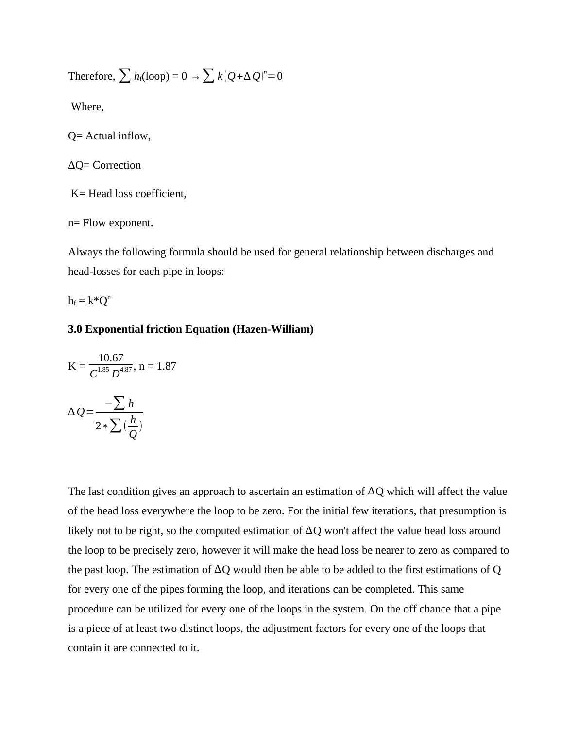
Therefore, ∑ hf(loop) = 0 →∑ k ( Q+∆ Q ) n =0
Where,
Q= Actual inflow,
ΔQ= Correction
K= Head loss coefficient,
n= Flow exponent.
Always the following formula should be used for general relationship between discharges and
head-losses for each pipe in loops:
hf = k*Qn
3.0 Exponential friction Equation (Hazen-William)
K = 10.67
C1.85 D4.87 , n = 1.87
∆ Q= −∑ h
2∗∑ ( h
Q )
The last condition gives an approach to ascertain an estimation of ∆Q which will affect the value
of the head loss everywhere the loop to be zero. For the initial few iterations, that presumption is
likely not to be right, so the computed estimation of ∆Q won't affect the value head loss around
the loop to be precisely zero, however it will make the head loss be nearer to zero as compared to
the past loop. The estimation of ∆Q would then be able to be added to the first estimations of Q
for every one of the pipes forming the loop, and iterations can be completed. This same
procedure can be utilized for every one of the loops in the system. On the off chance that a pipe
is a piece of at least two distinct loops, the adjustment factors for every one of the loops that
contain it are connected to it.