ANOVA with Replication Table Variations (6-8)
VerifiedAdded on 2019/10/18
|12
|7836
|268
Report
AI Summary
In this week's assignment, we explored two approaches to data analysis: the paired t-test and Analysis of Variance (ANOVA) tests. The paired t-test is used when examining mean differences between dependent variables, requiring at least interval-level data. ANOVA tests were introduced in three forms: one-factor ANOVA for comparing means from 3 or more groups, two-factor ANOVA without replication for comparing two variables with multiple measures, and two-factor ANOVA with replication for the same comparison but with a single measure per variable pair. Additionally, we examined interaction effects between variables and discussed effect size measures to determine the practical significance of findings. This includes eta squared values, which indicate whether the null hypothesis rejection was due to variable interaction or sample size.
Contribute Materials
Your contribution can guide someone’s learning journey. Share your
documents today.
Week 3 – Standardized Guidance – BUS 308: Statistics for Managers
After mastering this week’s material, you should
Understand:
o When the paired t-test is used.
o When the Analysis of Variance (ANOVA) test is used.
o How to calculate the effect size measure for each test.
o The differences between the one factor ANOVA, the two factor ANOVA without
replication, and the two factor ANOVA with replication.
o How to interpret the F statistic.
Be able to:
o Develop the null and alternate hypothesis statement for both the paired t-test and the
ANVOA tests from a research question.
o Use Excel to perform a paired t-test.
o Interpret the results of a paired t-test.
o Use Excel to perform ANOVA tests.
o Interpret the results of ANOVA tests.
o Calculate appropriate effect size measures for each test.
Continuing with Mean Differences
For Week Three, we will continue to look at mean differences. First we will look at dependent groups –
these exist when we take more than one measure from the subject (Tanner & Youssef-Morgan, 2013).
Comparing pre and post-test scores would be an example of dependent measures. This would be an
example of a 2 sample situation, we can also expand this analysis to 3 or more measures on the same
subjects. Then we will move on to testing means from 3 or more independent groups, where – as with
the t-tests we examined last week – we measure different subjects in each group (Lind, Marchel, &
Wathen, 2008).
Dependent/Paired t-test
Chapter 7 (Tanner & Youssef-Morgan, 2013) introduces the idea of a dependent variable – “repeated
measures of the same variable within the same group of subjects over time” (p. 164). This issue of
measuring the same subject over time or on two similar measures introduces some complexity into our
analysis. Due to differences in initial measures, differences in related measures are not due solely to the
factor being measured, but have a relationship to the initial results. For example, someone 6 feet tall can
generally jump higher than someone 5 feet tall; if we train both individuals in techniques to jump higher,
the taller person will still have an advantage – so treating the second measure as unrelated to the initial
starting point is not reasonable. There are several techniques available to us to take related measures
such as this into account.
This week we will look at the paired t-test, used when we have 2 measures on each subject. Chapter 7 in
the text (Tanner & Youssef-Morgan, 2013) also discusses the within-subjects F (AKA within-subjects
ANOVA). We will this later with the other forms of ANOVA introduced this week.
We start with another version of the t-test. Recall that last week we looked at the single sample t-test, the
2 sample t-test with equal variance and the 2 sample t-test with unequal variance (and noted how we can
use this version to perform a one sample t-test with no variance in the Ho sample). We now look at the
paired t-test. The uniqueness of this test is that for each subject in the sample we have two measures.
For example, determining if the difference in scores between a pre- and post-test for a course in statistics
is significant would be an example of a paired t-test situation. Another example would be how people did
in different subjects, for example is there a significant difference between scores in an English and
Secure Best Marks with AI Grader
Need help grading? Try our AI Grader for instant feedback on your assignments.
Statistics class? Note that we cannot just pair up measures – for example, attempting to pair a male and
female test score is NOT an example of a paired situation (Lind, Marchel, & Wathen, 2008).
The paired t-test t equals the mean difference between scores divided by the standard error of the mean
of these differences. The important information we are interested in for paired situations lies in the
difference between scores. By focusing on the differences rather than the actual scores, we are
controlling for the differences shown between subjects in the initial measure – how good or poor the initial
score was is not important, we only care about how much difference exists (Lind, Marchel, & Wathen,
2008).
Review: Choosing among the different versions of the t-test is fairly simple. If we have:
One group with only 1 measure: use the one-sample t-test (or trick excel by using the two sample
unequal variance t-test with one variable equaling only the hypothesized value)
Two groups with the same measure for each: use either the equal or unequal variance 2 sample
t-test
One group that has 2 measures on each subject: use the paired t-test.
Excel Example
In our equal pay case, we do have two measures for each employee that we could compare for mean
equality – the salary and the midpoint. Each is measured in dollar units, so they are comparable. There
are a couple of tests we could make. We could compare everyone’s salary and midpoint to see if the
average were equal or not. We could also look at each gender individually – that is, are the male and
female salary averages equal to their respective midpoint averages? We can also note that since none of
the other variables have the same measurement scale, there are no other paired comparisons that we
could make.
Question: Is the female mean salary greater than the female mean midpoint?
Step 1: Ho: Female mean salary <= female mean midpoint (Note: Remember that the null always has to
have the = sign in it, since our question did not imply an equality, the question represents the alternative
and we back into the null as the opposite statement.)
Ha: Female mean salary > female mean midpoint (Note: since we have a one way question that does not
include an equal term in the question, the alternate is generally expresses the question. If the question
had been mean salary greater than or equal to the mean midpoint, the null would have expressed the
question: Ho: mean salary => mean midpoint, and Ha: mean salary < mean midpoint.)
Step 2: Test to use: Paired t-test. (Note: we have two measures – salary and midpoint – on each person,
thus it is paired data.)
Step 3: Decision rule: If the p-value is < 0.05 and the t statistic is in the left side of the its
distribution/mean, then we reject the null hypothesis. (Note: since we have a one tail test, we need to
ensure that the calculated salary mean statistic is in fact less than the midpoint mean; this translates to a
negative t-value – our hint as to which side of the curve to use is given by arrow in the alternate pointing
to the left side of the curve. In order for everything to line up correctly, the t-test needs to enter the
variables in the same order as listed in the hypothesis statements.)
Step 4: Execution - Excel solution: Copy and paste the female salary and midpoint columns to a new
spreadsheet (or to the spreadsheet with the question on the assignment file) – be sure to include the
variable names at the top of each column. In the data, Data Analysis button select the T-test: Paired Two
Sample for Means option. In the variable 1 range, enter the salary range; in the variable 2 range, enter
the midpoint range. Click on the labels box (if you have labels in the input ranges). Click on the Output
Range button and then enter the upper left corner cell where you want the output to go. Clicking OK will
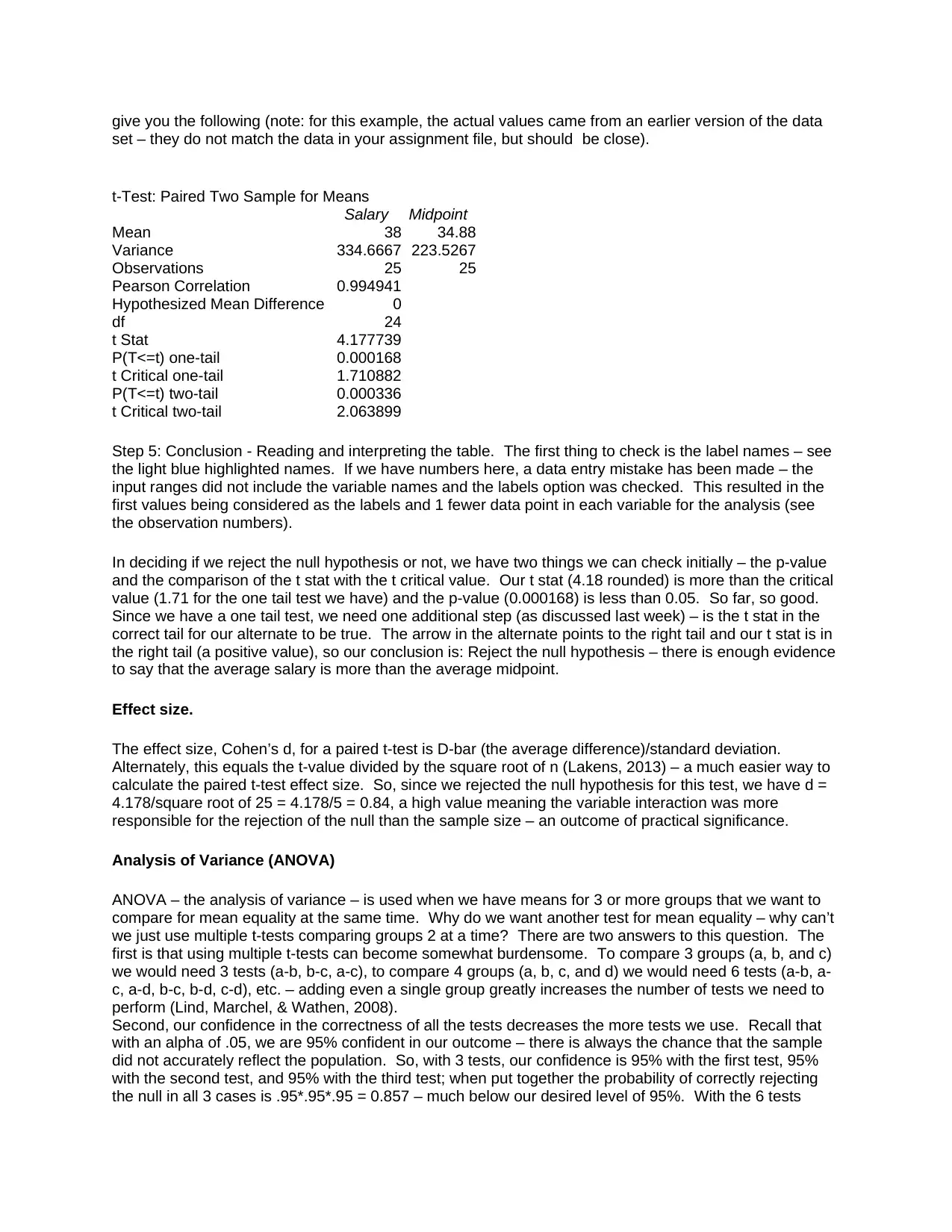
give you the following (note: for this example, the actual values came from an earlier version of the data
set – they do not match the data in your assignment file, but should be close).
t-Test: Paired Two Sample for Means
Salary Midpoint
Mean 38 34.88
Variance 334.6667 223.5267
Observations 25 25
Pearson Correlation 0.994941
Hypothesized Mean Difference 0
df 24
t Stat 4.177739
P(T<=t) one-tail 0.000168
t Critical one-tail 1.710882
P(T<=t) two-tail 0.000336
t Critical two-tail 2.063899
Step 5: Conclusion - Reading and interpreting the table. The first thing to check is the label names – see
the light blue highlighted names. If we have numbers here, a data entry mistake has been made – the
input ranges did not include the variable names and the labels option was checked. This resulted in the
first values being considered as the labels and 1 fewer data point in each variable for the analysis (see
the observation numbers).
In deciding if we reject the null hypothesis or not, we have two things we can check initially – the p-value
and the comparison of the t stat with the t critical value. Our t stat (4.18 rounded) is more than the critical
value (1.71 for the one tail test we have) and the p-value (0.000168) is less than 0.05. So far, so good.
Since we have a one tail test, we need one additional step (as discussed last week) – is the t stat in the
correct tail for our alternate to be true. The arrow in the alternate points to the right tail and our t stat is in
the right tail (a positive value), so our conclusion is: Reject the null hypothesis – there is enough evidence
to say that the average salary is more than the average midpoint.
Effect size.
The effect size, Cohen’s d, for a paired t-test is D-bar (the average difference)/standard deviation.
Alternately, this equals the t-value divided by the square root of n (Lakens, 2013) – a much easier way to
calculate the paired t-test effect size. So, since we rejected the null hypothesis for this test, we have d =
4.178/square root of 25 = 4.178/5 = 0.84, a high value meaning the variable interaction was more
responsible for the rejection of the null than the sample size – an outcome of practical significance.
Analysis of Variance (ANOVA)
ANOVA – the analysis of variance – is used when we have means for 3 or more groups that we want to
compare for mean equality at the same time. Why do we want another test for mean equality – why can’t
we just use multiple t-tests comparing groups 2 at a time? There are two answers to this question. The
first is that using multiple t-tests can become somewhat burdensome. To compare 3 groups (a, b, and c)
we would need 3 tests (a-b, b-c, a-c), to compare 4 groups (a, b, c, and d) we would need 6 tests (a-b, a-
c, a-d, b-c, b-d, c-d), etc. – adding even a single group greatly increases the number of tests we need to
perform (Lind, Marchel, & Wathen, 2008).
Second, our confidence in the correctness of all the tests decreases the more tests we use. Recall that
with an alpha of .05, we are 95% confident in our outcome – there is always the chance that the sample
did not accurately reflect the population. So, with 3 tests, our confidence is 95% with the first test, 95%
with the second test, and 95% with the third test; when put together the probability of correctly rejecting
the null in all 3 cases is .95*.95*.95 = 0.857 – much below our desired level of 95%. With the 6 tests
needed for the 4 group comparison, our overall percent becomes 0.735. In order to keep our desired
confidence in the results we need to perform all of the comparison in one test – the ANOVA (Lind,
Marchel, & Wathen, 2008).
ANOVA tests mean equality by comparing the variance of the entire data set with the average variance of
the individual groups. Therefore, it assumes equal population variances for each group. This assumption
is critical, and should always be verified before using the results of an ANOVA analysis. If you have more
than two groups, compare the largest and smallest variances with the F test (discussed in week 2 for
verifying equal variances in choosing the appropriate 2 sample t-test to use) outcome – if they are not
significantly different, none of the others will be (Lind, Marchel, & Wathen, 2008).
Just how does testing variance equality tell us that means are equal? The underlying logic says that if (1)
the groups come from populations having equal variances AND (2) equal means, then the different
groups will overlap each other if graphed and the entire data set should have the same mean and
variance as each of the samples (within statistical sampling error). If this is true, then the resulting F will
be small. If however, the groups have equal variances and UNEQUAL means, they will be spread out
rather than overlap and the variance of the overall group will be greater than the average variance for the
individual groups and F will be large (Lind, Marchel, & Wathen, 2008).
While ANOVA can be used for 2 groups (the results will be identical to those obtained with the two
sample equal variance t-test), by convention we use the t for two groups and ANOVA for 3 or more
groups (Lind, Marchel, & Wathen, 2008). In our equal pay example, if we think that age is a reason for
differing salaries among the grades, we could use ANOVA to see if the average ages for each grade level
are different.
ANOVA requires that the different populations being tested have the same variance. This is tested by
using the F-test introduced last week. By testing the sample with the largest variance against the sample
with the smallest variance, we can see if the variances are statistically equal or not. If the extremes are
not significantly different, values between them will also not differ (Lind, Marchel, & Wathen, 2008).
Real Life Example
One of the course instructors was charged with creating and starting supervisory training classes for a
company, The initial proposed 5-day basic supervisory program in a single week met with some initial
resistance, as company had never done that before, and the Vice President of Human Resources did not
think the managers would accept having their supervisors gone for this period. So, a test was offered.
The training would be initially scheduled in 3 different formats, and the managers could pick which they
wanted their supervisors to attend – once a week, twice a week, or the full week. At the end, the pre- and
post-test scores – and change in scores - were evaluated to see if format made a difference. The
ANOVA was used to verify that the pre-test results were the same – that is, the average knowledge level
of supervisors entering the program was not different between the sessions. The paired t-tests showed
that learning occurred in each session. At the end, the ANOVA was again used to see if a difference
existed between the formats. It did, and this evidence was used to schedule the remainder of the classes
in the full 5 day format.
Types of ANOVA tests
Just as the t-test has 3 versions (one-sample, two-sample, and paired) to choose from, ANOVA also has
several choices. The three approaches described in the text match those of the choices that Excel offers
– chapter 5’s one way ANVOA is the same as Excel’s ANOVA single factor; chapter 6’s Factorial ANOVA
is the same as Excel’s ANOVA: two factor with replication. The authors (Tanner & Youssef-Morgan,
2013) make a somewhat confusing comment on p. 184: “Dependent groups ANOVA is not one of the
options Excel offers.” The Excel option 2 factor ANOVA without replication, when used with each
example in chapter 7 produce the same results with some additional information – it provides information
to test more than the dependent measures across the same subject. We will discuss this in more detail
Secure Best Marks with AI Grader
Need help grading? Try our AI Grader for instant feedback on your assignments.
below.
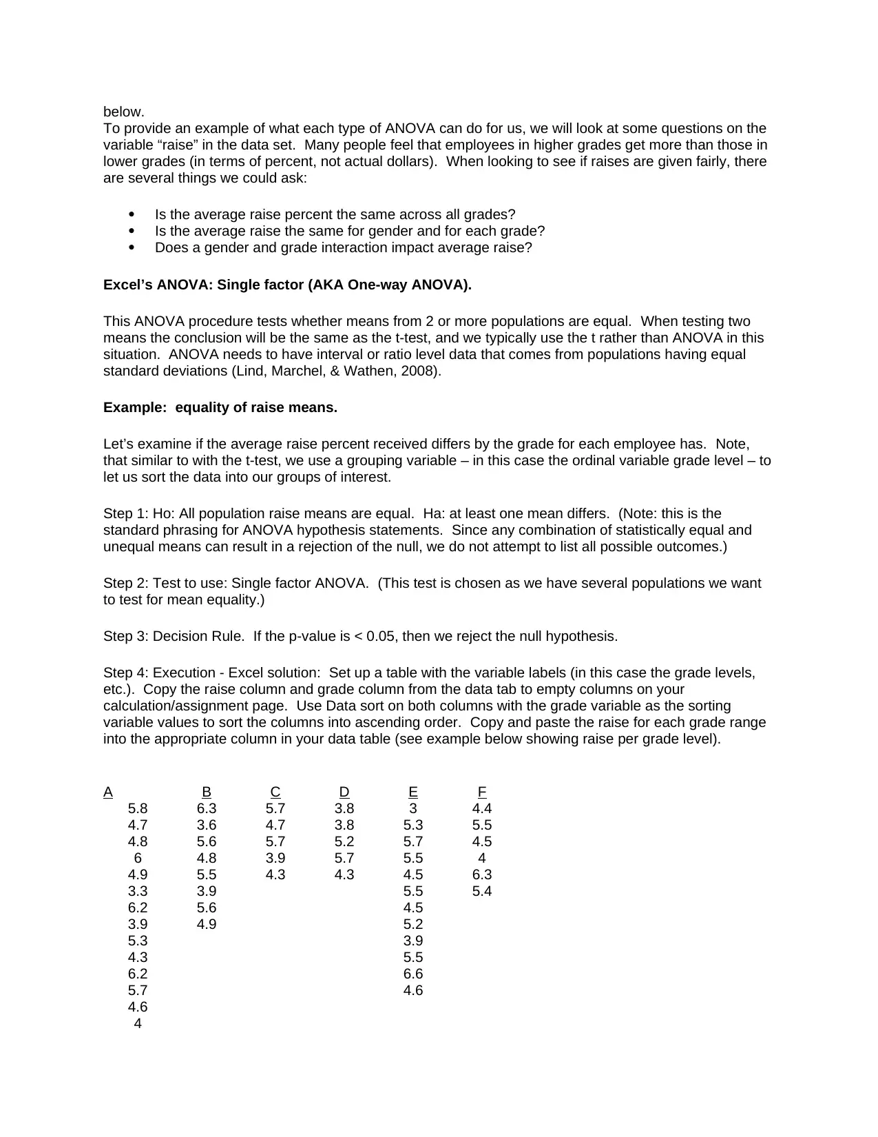
To provide an example of what each type of ANOVA can do for us, we will look at some questions on the
variable “raise” in the data set. Many people feel that employees in higher grades get more than those in
lower grades (in terms of percent, not actual dollars). When looking to see if raises are given fairly, there
are several things we could ask:
Is the average raise percent the same across all grades?
Is the average raise the same for gender and for each grade?
Does a gender and grade interaction impact average raise?
Excel’s ANOVA: Single factor (AKA One-way ANOVA).
This ANOVA procedure tests whether means from 2 or more populations are equal. When testing two
means the conclusion will be the same as the t-test, and we typically use the t rather than ANOVA in this
situation. ANOVA needs to have interval or ratio level data that comes from populations having equal
standard deviations (Lind, Marchel, & Wathen, 2008).
Example: equality of raise means.
Let’s examine if the average raise percent received differs by the grade for each employee has. Note,
that similar to with the t-test, we use a grouping variable – in this case the ordinal variable grade level – to
let us sort the data into our groups of interest.
Step 1: Ho: All population raise means are equal. Ha: at least one mean differs. (Note: this is the
standard phrasing for ANOVA hypothesis statements. Since any combination of statistically equal and
unequal means can result in a rejection of the null, we do not attempt to list all possible outcomes.)
Step 2: Test to use: Single factor ANOVA. (This test is chosen as we have several populations we want
to test for mean equality.)
Step 3: Decision Rule. If the p-value is < 0.05, then we reject the null hypothesis.
Step 4: Execution - Excel solution: Set up a table with the variable labels (in this case the grade levels,
etc.). Copy the raise column and grade column from the data tab to empty columns on your
calculation/assignment page. Use Data sort on both columns with the grade variable as the sorting
variable values to sort the columns into ascending order. Copy and paste the raise for each grade range
into the appropriate column in your data table (see example below showing raise per grade level).
A B C D E F
5.8 6.3 5.7 3.8 3 4.4
4.7 3.6 4.7 3.8 5.3 5.5
4.8 5.6 5.7 5.2 5.7 4.5
6 4.8 3.9 5.7 5.5 4
4.9 5.5 4.3 4.3 4.5 6.3
3.3 3.9 5.5 5.4
6.2 5.6 4.5
3.9 4.9 5.2
5.3 3.9
4.3 5.5
6.2 6.6
5.7 4.6
4.6
4
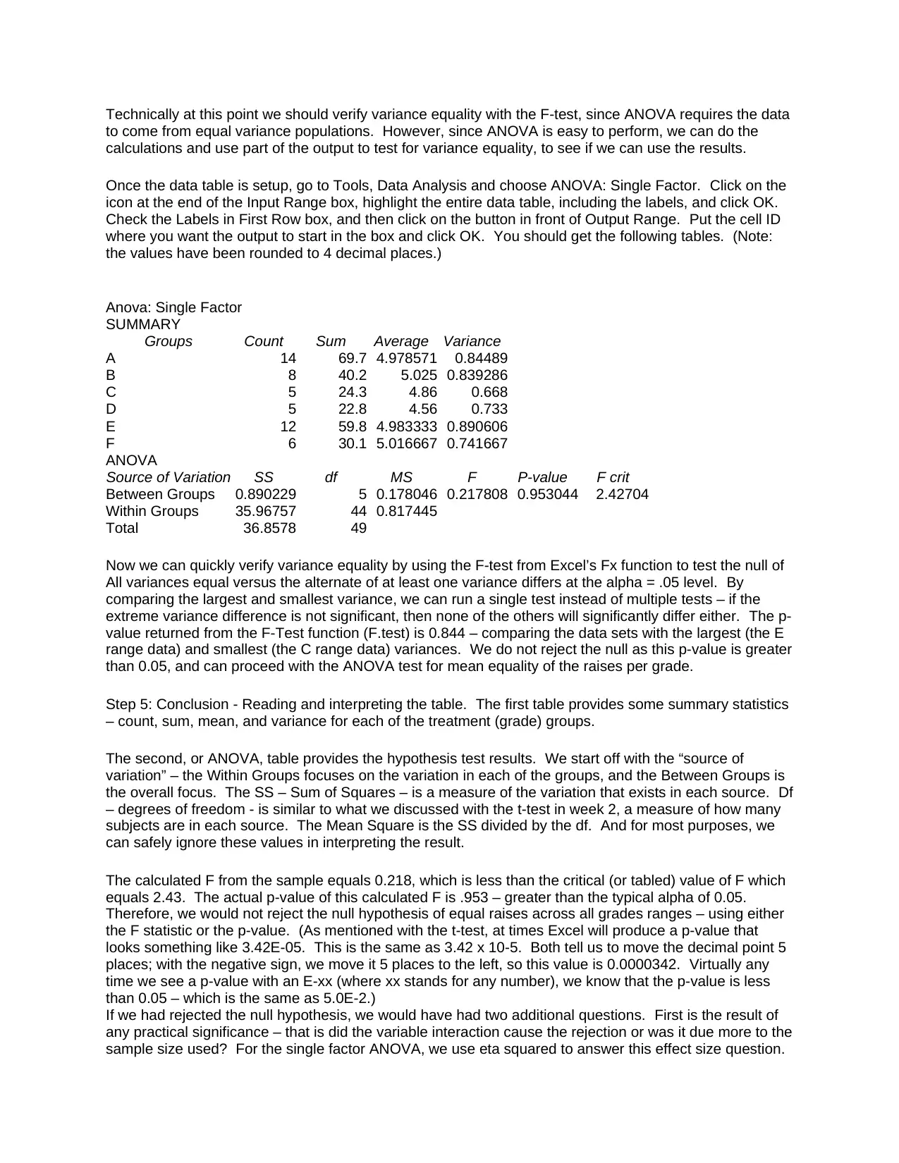
Technically at this point we should verify variance equality with the F-test, since ANOVA requires the data
to come from equal variance populations. However, since ANOVA is easy to perform, we can do the
calculations and use part of the output to test for variance equality, to see if we can use the results.
Once the data table is setup, go to Tools, Data Analysis and choose ANOVA: Single Factor. Click on the
icon at the end of the Input Range box, highlight the entire data table, including the labels, and click OK.
Check the Labels in First Row box, and then click on the button in front of Output Range. Put the cell ID
where you want the output to start in the box and click OK. You should get the following tables. (Note:
the values have been rounded to 4 decimal places.)
Anova: Single Factor
SUMMARY
Groups Count Sum Average Variance
A 14 69.7 4.978571 0.84489
B 8 40.2 5.025 0.839286
C 5 24.3 4.86 0.668
D 5 22.8 4.56 0.733
E 12 59.8 4.983333 0.890606
F 6 30.1 5.016667 0.741667
ANOVA
Source of Variation SS df MS F P-value F crit
Between Groups 0.890229 5 0.178046 0.217808 0.953044 2.42704
Within Groups 35.96757 44 0.817445
Total 36.8578 49
Now we can quickly verify variance equality by using the F-test from Excel’s Fx function to test the null of
All variances equal versus the alternate of at least one variance differs at the alpha = .05 level. By
comparing the largest and smallest variance, we can run a single test instead of multiple tests – if the
extreme variance difference is not significant, then none of the others will significantly differ either. The p-
value returned from the F-Test function (F.test) is 0.844 – comparing the data sets with the largest (the E
range data) and smallest (the C range data) variances. We do not reject the null as this p-value is greater
than 0.05, and can proceed with the ANOVA test for mean equality of the raises per grade.
Step 5: Conclusion - Reading and interpreting the table. The first table provides some summary statistics
– count, sum, mean, and variance for each of the treatment (grade) groups.
The second, or ANOVA, table provides the hypothesis test results. We start off with the “source of
variation” – the Within Groups focuses on the variation in each of the groups, and the Between Groups is
the overall focus. The SS – Sum of Squares – is a measure of the variation that exists in each source. Df
– degrees of freedom - is similar to what we discussed with the t-test in week 2, a measure of how many
subjects are in each source. The Mean Square is the SS divided by the df. And for most purposes, we
can safely ignore these values in interpreting the result.
The calculated F from the sample equals 0.218, which is less than the critical (or tabled) value of F which
equals 2.43. The actual p-value of this calculated F is .953 – greater than the typical alpha of 0.05.
Therefore, we would not reject the null hypothesis of equal raises across all grades ranges – using either
the F statistic or the p-value. (As mentioned with the t-test, at times Excel will produce a p-value that
looks something like 3.42E-05. This is the same as 3.42 x 10⁻⁵. Both tell us to move the decimal point 5
places; with the negative sign, we move it 5 places to the left, so this value is 0.0000342. Virtually any
time we see a p-value with an E-xx (where xx stands for any number), we know that the p-value is less
than 0.05 – which is the same as 5.0E-2.)
If we had rejected the null hypothesis, we would have had two additional questions. First is the result of
any practical significance – that is did the variable interaction cause the rejection or was it due more to the
sample size used? For the single factor ANOVA, we use eta squared to answer this effect size question.
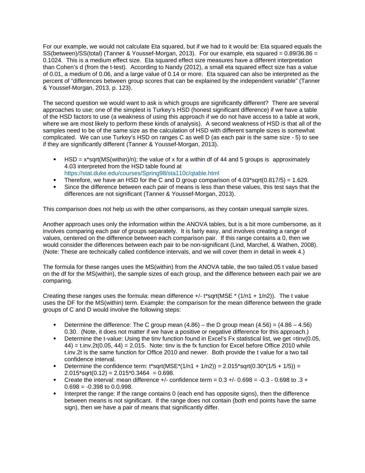
For our example, we would not calculate Eta squared, but if we had to it would be: Eta squared equals the
SS(between)/SS(total) (Tanner & Youssef-Morgan, 2013). For our example, eta squared = 0.89/36.86 =
0.1024. This is a medium effect size. Eta squared effect size measures have a different interpretation
than Cohen’s d (from the t-test). According to Nandy (2012), a small eta squared effect size has a value
of 0.01, a medium of 0.06, and a large value of 0.14 or more. Eta squared can also be interpreted as the
percent of “differences between group scores that can be explained by the independent variable” (Tanner
& Youssef-Morgan, 2013, p. 123).
The second question we would want to ask is which groups are significantly different? There are several
approaches to use; one of the simplest is Turkey’s HSD (honest significant difference) if we have a table
of the HSD factors to use (a weakness of using this approach if we do not have access to a table at work,
where we are most likely to perform these kinds of analysis). A second weakness of HSD is that all of the
samples need to be of the same size as the calculation of HSD with different sample sizes is somewhat
complicated. We can use Turkey’s HSD on ranges C as well D (as each pair is the same size - 5) to see
if they are significantly different (Tanner & Youssef-Morgan, 2013).
HSD = x*sqrt(MS(within)/n); the value of x for a within df of 44 and 5 groups is approximately
4.03 interpreted from the HSD table found at
https://stat.duke.edu/courses/Spring98/sta110c/qtable.html
Therefore, we have an HSD for the C and D group comparison of 4.03*sqrt(0.817/5) = 1.629.
Since the difference between each pair of means is less than these values, this test says that the
differences are not significant (Tanner & Youssef-Morgan, 2013).
This comparison does not help us with the other comparisons, as they contain unequal sample sizes.
Another approach uses only the information within the ANOVA tables, but is a bit more cumbersome, as it
involves comparing each pair of groups separately. It is fairly easy, and involves creating a range of
values, centered on the difference between each comparison pair. If this range contains a 0, then we
would consider the differences between each pair to be non-significant (Lind, Marchel, & Wathen, 2008).
(Note: These are technically called confidence intervals, and we will cover them in detail in week 4.)
The formula for these ranges uses the MS(within) from the ANOVA table, the two tailed.05 t value based
on the df for the MS(within), the sample sizes of each group, and the difference between each pair we are
comparing.
Creating these ranges uses the formula: mean difference +/- t*sqrt(MSE * (1/n1 + 1/n2)). The t value
uses the DF for the MS(within) term. Example: the comparison for the mean difference between the grade
groups of C and D would involve the following steps:
Determine the difference: The C group mean (4.86) – the D group mean (4.56) = (4.86 – 4.56)
0.30. (Note, it does not matter if we have a positive or negative difference for this approach.)
Determine the t-value: Using the tinv function found in Excel’s Fx statistical list, we get =tinv(0.05,
44) = t.inv.2t(0.05, 44) = 2.015. Note: tinv is the fx function for Excel before Office 2010 while
t.inv.2t is the same function for Office 2010 and newer. Both provide the t value for a two tail
confidence interval.
Determine the confidence term: t*sqrt(MSE*(1/n1 + 1/n2)) = 2.015*sqrt(0.30*(1/5 + 1/5)) =
2.015*sqrt(0.12) = 2.015*0.3464 = 0.698.
Create the interval: mean difference +/- confidence term = 0.3 +/- 0.698 = -0.3 - 0.698 to .3 +
0.698 = -0.398 to 0.0.998.
Interpret the range: If the range contains 0 (each end has opposite signs), then the difference
between means is not significant. If the range does not contain (both end points have the same
sign), then we have a pair of means that significantly differ.
Paraphrase This Document
Need a fresh take? Get an instant paraphrase of this document with our AI Paraphraser
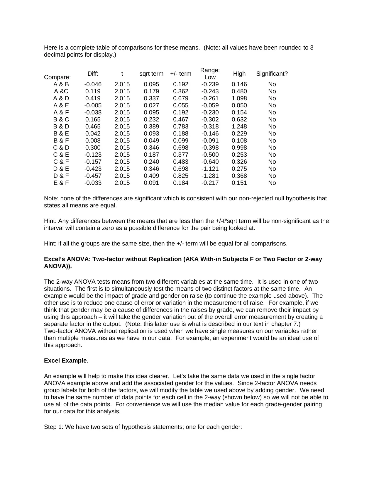
Here is a complete table of comparisons for these means. (Note: all values have been rounded to 3
decimal points for display.)
Compare: Diff: t sqrt term +/- term Range:
Low High Significant?
A & B -0.046 2.015 0.095 0.192 -0.239 0.146 No
A &C 0.119 2.015 0.179 0.362 -0.243 0.480 No
A & D 0.419 2.015 0.337 0.679 -0.261 1.098 No
A & E -0.005 2.015 0.027 0.055 -0.059 0.050 No
A & F -0.038 2.015 0.095 0.192 -0.230 0.154 No
B & C 0.165 2.015 0.232 0.467 -0.302 0.632 No
B & D 0.465 2.015 0.389 0.783 -0.318 1.248 No
B & E 0.042 2.015 0.093 0.188 -0.146 0.229 No
B & F 0.008 2.015 0.049 0.099 -0.091 0.108 No
C & D 0.300 2.015 0.346 0.698 -0.398 0.998 No
C & E -0.123 2.015 0.187 0.377 -0.500 0.253 No
C & F -0.157 2.015 0.240 0.483 -0.640 0.326 No
D & E -0.423 2.015 0.346 0.698 -1.121 0.275 No
D & F -0.457 2.015 0.409 0.825 -1.281 0.368 No
E & F -0.033 2.015 0.091 0.184 -0.217 0.151 No
Note: none of the differences are significant which is consistent with our non-rejected null hypothesis that
states all means are equal.
Hint: Any differences between the means that are less than the +/-t*sqrt term will be non-significant as the
interval will contain a zero as a possible difference for the pair being looked at.
Hint: if all the groups are the same size, then the +/- term will be equal for all comparisons.
Excel’s ANOVA: Two-factor without Replication (AKA With-in Subjects F or Two Factor or 2-way
ANOVA)).
The 2-way ANOVA tests means from two different variables at the same time. It is used in one of two
situations. The first is to simultaneously test the means of two distinct factors at the same time. An
example would be the impact of grade and gender on raise (to continue the example used above). The
other use is to reduce one cause of error or variation in the measurement of raise. For example, if we
think that gender may be a cause of differences in the raises by grade, we can remove their impact by
using this approach – it will take the gender variation out of the overall error measurement by creating a
separate factor in the output. (Note: this latter use is what is described in our text in chapter 7.)
Two-factor ANOVA without replication is used when we have single measures on our variables rather
than multiple measures as we have in our data. For example, an experiment would be an ideal use of
this approach.
Excel Example.
An example will help to make this idea clearer. Let’s take the same data we used in the single factor
ANOVA example above and add the associated gender for the values. Since 2-factor ANOVA needs
group labels for both of the factors, we will modify the table we used above by adding gender. We need
to have the same number of data points for each cell in the 2-way (shown below) so we will not be able to
use all of the data points. For convenience we will use the median value for each grade-gender pairing
for our data for this analysis.
Step 1: We have two sets of hypothesis statements; one for each gender:
Ho: All population raise means across grade groups are equal. Ha: At least one mean differs.
Ho: All population raise means across gender groups are equal. Ha: At least one mean differs.
(Note: we would only have this hypothesis pair if we were interested in testing equality across
gender; if we merely wanted to remove gender as a possible source of variation across the grade
groups we would not test gender.)
Step 2: Test to use: 2-factor Anova without replication. (This test is chosen as we have 2 group factors
we want to test for mean equality, and only a single measure for each variable pair.)
Step 3: Decision Rule. If the p-value is < 0.05, then we reject the null hypothesis.
Step 4: Execution - Excel solution: Set up a table with the variable labels (in this case the grade labels
– .A, B, etc. and gender labels). For this situation we need to decide what data values to use, as we have
quite a few values to choose from; other times we will have only a single measurement from an
experiment. The median value from group is a way to get the most representative value, without being
swayed by extreme values.
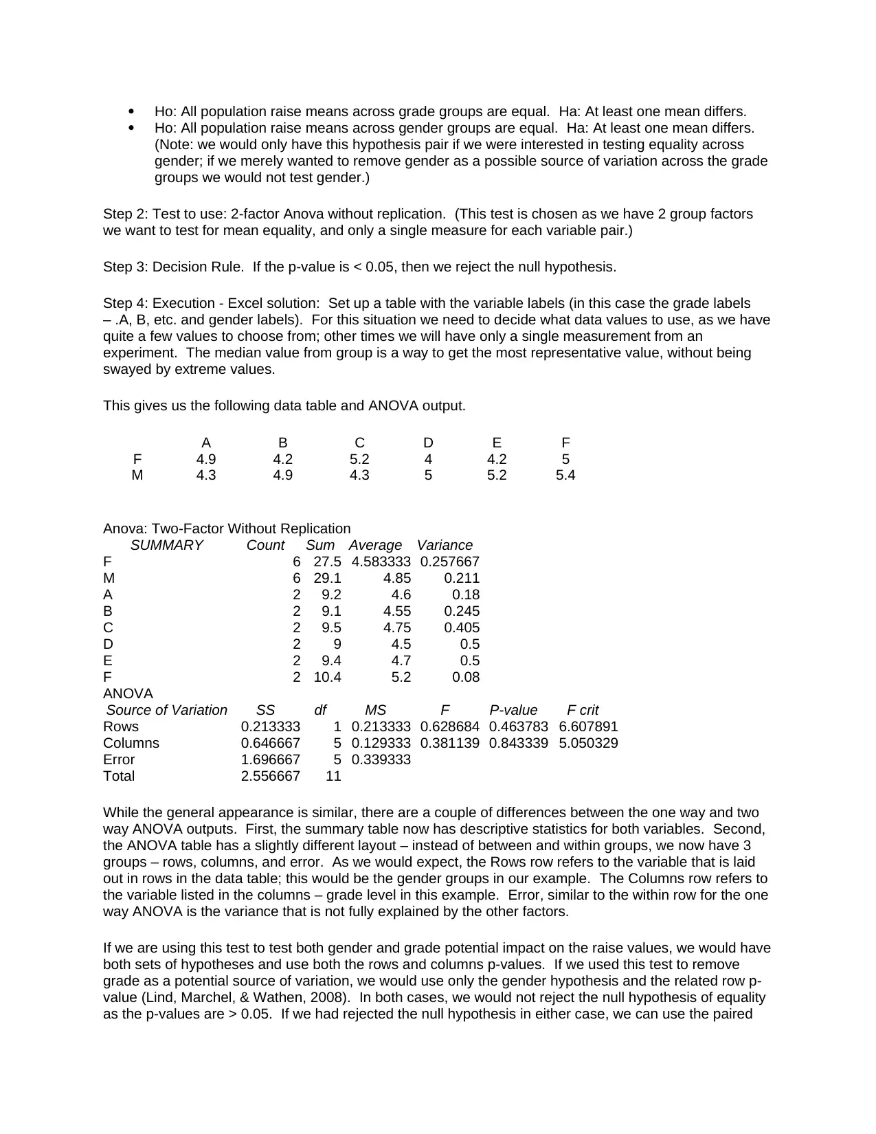
This gives us the following data table and ANOVA output.
A B C D E F
F 4.9 4.2 5.2 4 4.2 5
M 4.3 4.9 4.3 5 5.2 5.4
Anova: Two-Factor Without Replication
SUMMARY Count Sum Average Variance
F 6 27.5 4.583333 0.257667
M 6 29.1 4.85 0.211
A 2 9.2 4.6 0.18
B 2 9.1 4.55 0.245
C 2 9.5 4.75 0.405
D 2 9 4.5 0.5
E 2 9.4 4.7 0.5
F 2 10.4 5.2 0.08
ANOVA
Source of Variation SS df MS F P-value F crit
Rows 0.213333 1 0.213333 0.628684 0.463783 6.607891
Columns 0.646667 5 0.129333 0.381139 0.843339 5.050329
Error 1.696667 5 0.339333
Total 2.556667 11
While the general appearance is similar, there are a couple of differences between the one way and two
way ANOVA outputs. First, the summary table now has descriptive statistics for both variables. Second,
the ANOVA table has a slightly different layout – instead of between and within groups, we now have 3
groups – rows, columns, and error. As we would expect, the Rows row refers to the variable that is laid
out in rows in the data table; this would be the gender groups in our example. The Columns row refers to
the variable listed in the columns – grade level in this example. Error, similar to the within row for the one
way ANOVA is the variance that is not fully explained by the other factors.
If we are using this test to test both gender and grade potential impact on the raise values, we would have
both sets of hypotheses and use both the rows and columns p-values. If we used this test to remove
grade as a potential source of variation, we would use only the gender hypothesis and the related row p-
value (Lind, Marchel, & Wathen, 2008). In both cases, we would not reject the null hypothesis of equality
as the p-values are > 0.05. If we had rejected the null hypothesis in either case, we can use the paired
Ho: All population raise means across gender groups are equal. Ha: At least one mean differs.
(Note: we would only have this hypothesis pair if we were interested in testing equality across
gender; if we merely wanted to remove gender as a possible source of variation across the grade
groups we would not test gender.)
Step 2: Test to use: 2-factor Anova without replication. (This test is chosen as we have 2 group factors
we want to test for mean equality, and only a single measure for each variable pair.)
Step 3: Decision Rule. If the p-value is < 0.05, then we reject the null hypothesis.
Step 4: Execution - Excel solution: Set up a table with the variable labels (in this case the grade labels
– .A, B, etc. and gender labels). For this situation we need to decide what data values to use, as we have
quite a few values to choose from; other times we will have only a single measurement from an
experiment. The median value from group is a way to get the most representative value, without being
swayed by extreme values.
This gives us the following data table and ANOVA output.
A B C D E F
F 4.9 4.2 5.2 4 4.2 5
M 4.3 4.9 4.3 5 5.2 5.4
Anova: Two-Factor Without Replication
SUMMARY Count Sum Average Variance
F 6 27.5 4.583333 0.257667
M 6 29.1 4.85 0.211
A 2 9.2 4.6 0.18
B 2 9.1 4.55 0.245
C 2 9.5 4.75 0.405
D 2 9 4.5 0.5
E 2 9.4 4.7 0.5
F 2 10.4 5.2 0.08
ANOVA
Source of Variation SS df MS F P-value F crit
Rows 0.213333 1 0.213333 0.628684 0.463783 6.607891
Columns 0.646667 5 0.129333 0.381139 0.843339 5.050329
Error 1.696667 5 0.339333
Total 2.556667 11
While the general appearance is similar, there are a couple of differences between the one way and two
way ANOVA outputs. First, the summary table now has descriptive statistics for both variables. Second,
the ANOVA table has a slightly different layout – instead of between and within groups, we now have 3
groups – rows, columns, and error. As we would expect, the Rows row refers to the variable that is laid
out in rows in the data table; this would be the gender groups in our example. The Columns row refers to
the variable listed in the columns – grade level in this example. Error, similar to the within row for the one
way ANOVA is the variance that is not fully explained by the other factors.
If we are using this test to test both gender and grade potential impact on the raise values, we would have
both sets of hypotheses and use both the rows and columns p-values. If we used this test to remove
grade as a potential source of variation, we would use only the gender hypothesis and the related row p-
value (Lind, Marchel, & Wathen, 2008). In both cases, we would not reject the null hypothesis of equality
as the p-values are > 0.05. If we had rejected the null hypothesis in either case, we can use the paired
comparison ranges that were demonstrated for the 1-way ANOVA to determine which sets of means
differ. We would use the MS(error) term for both determining the t-value and in the confidence range
calculation rather than the MS(within) that was used in the 1-way ANOVA.
The effect size measure for a 2-factor ANOVA without replication is generally the same as with the single
factor ANOVA. For each variable it would be eta squared = SS(for variable) divided by the SS(total)
value (Tanner & Youssef-Morgan, 2013).
Excel’s ANOVA: Two-factor with Replication (AKA Factorial ANOVA). This form of the ANOVA test
is somewhat different than the previous two forms. While it can test for mean equality (or differences),
this is not its primary purpose. The main purpose is to look at the impact of interaction between variables
– that is do the results show different patterns when graphed? Interaction means the variables react
differently at different measurement levels (Lind, Marchel, & Wathen, 2008).
As we have done with the other forms, let’s look at the output of this form to help us understand what it
does. With replication, we have multiple data points for each of the cells in the 2-way (with replication)
data set up. So, keeping with the gender and grade impact on raise, the data table for this test would look
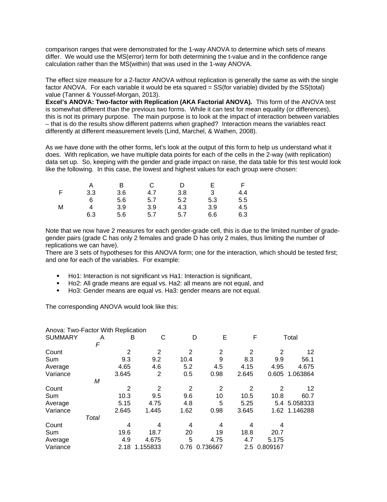
like the following. In this case, the lowest and highest values for each group were chosen:
A B C D E F
F 3.3 3.6 4.7 3.8 3 4.4
6 5.6 5.7 5.2 5.3 5.5
M 4 3.9 3.9 4.3 3.9 4.5
6.3 5.6 5.7 5.7 6.6 6.3
Note that we now have 2 measures for each gender-grade cell, this is due to the limited number of grade-
gender pairs (grade C has only 2 females and grade D has only 2 males, thus limiting the number of
replications we can have).
There are 3 sets of hypotheses for this ANOVA form; one for the interaction, which should be tested first;
and one for each of the variables. For example:
Ho1: Interaction is not significant vs Ha1: Interaction is significant,
Ho2: All grade means are equal vs. Ha2: all means are not equal, and
Ho3: Gender means are equal vs. Ha3: gender means are not equal.
The corresponding ANOVA would look like this:
Anova: Two-Factor With Replication
SUMMARY A B C D E F Total
F
Count 2 2 2 2 2 2 12
Sum 9.3 9.2 10.4 9 8.3 9.9 56.1
Average 4.65 4.6 5.2 4.5 4.15 4.95 4.675
Variance 3.645 2 0.5 0.98 2.645 0.605 1.063864
M
Count 2 2 2 2 2 2 12
Sum 10.3 9.5 9.6 10 10.5 10.8 60.7
Average 5.15 4.75 4.8 5 5.25 5.4 5.058333
Variance 2.645 1.445 1.62 0.98 3.645 1.62 1.146288
Total
Count 4 4 4 4 4 4
Sum 19.6 18.7 20 19 18.8 20.7
Average 4.9 4.675 5 4.75 4.7 5.175
Variance 2.18 1.155833 0.76 0.736667 2.5 0.809167
differ. We would use the MS(error) term for both determining the t-value and in the confidence range
calculation rather than the MS(within) that was used in the 1-way ANOVA.
The effect size measure for a 2-factor ANOVA without replication is generally the same as with the single
factor ANOVA. For each variable it would be eta squared = SS(for variable) divided by the SS(total)
value (Tanner & Youssef-Morgan, 2013).
Excel’s ANOVA: Two-factor with Replication (AKA Factorial ANOVA). This form of the ANOVA test
is somewhat different than the previous two forms. While it can test for mean equality (or differences),
this is not its primary purpose. The main purpose is to look at the impact of interaction between variables
– that is do the results show different patterns when graphed? Interaction means the variables react
differently at different measurement levels (Lind, Marchel, & Wathen, 2008).
As we have done with the other forms, let’s look at the output of this form to help us understand what it
does. With replication, we have multiple data points for each of the cells in the 2-way (with replication)
data set up. So, keeping with the gender and grade impact on raise, the data table for this test would look
like the following. In this case, the lowest and highest values for each group were chosen:
A B C D E F
F 3.3 3.6 4.7 3.8 3 4.4
6 5.6 5.7 5.2 5.3 5.5
M 4 3.9 3.9 4.3 3.9 4.5
6.3 5.6 5.7 5.7 6.6 6.3
Note that we now have 2 measures for each gender-grade cell, this is due to the limited number of grade-
gender pairs (grade C has only 2 females and grade D has only 2 males, thus limiting the number of
replications we can have).
There are 3 sets of hypotheses for this ANOVA form; one for the interaction, which should be tested first;
and one for each of the variables. For example:
Ho1: Interaction is not significant vs Ha1: Interaction is significant,
Ho2: All grade means are equal vs. Ha2: all means are not equal, and
Ho3: Gender means are equal vs. Ha3: gender means are not equal.
The corresponding ANOVA would look like this:
Anova: Two-Factor With Replication
SUMMARY A B C D E F Total
F
Count 2 2 2 2 2 2 12
Sum 9.3 9.2 10.4 9 8.3 9.9 56.1
Average 4.65 4.6 5.2 4.5 4.15 4.95 4.675
Variance 3.645 2 0.5 0.98 2.645 0.605 1.063864
M
Count 2 2 2 2 2 2 12
Sum 10.3 9.5 9.6 10 10.5 10.8 60.7
Average 5.15 4.75 4.8 5 5.25 5.4 5.058333
Variance 2.645 1.445 1.62 0.98 3.645 1.62 1.146288
Total
Count 4 4 4 4 4 4
Sum 19.6 18.7 20 19 18.8 20.7
Average 4.9 4.675 5 4.75 4.7 5.175
Variance 2.18 1.155833 0.76 0.736667 2.5 0.809167
Secure Best Marks with AI Grader
Need help grading? Try our AI Grader for instant feedback on your assignments.
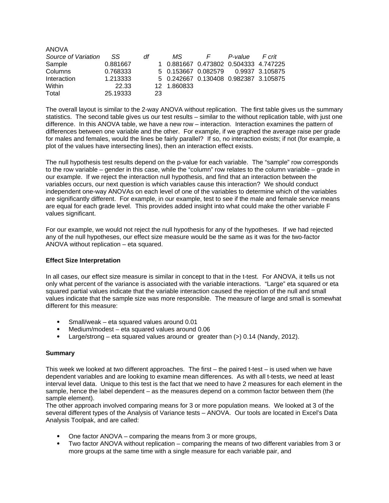
ANOVA
Source of Variation SS df MS F P-value F crit
Sample 0.881667 1 0.881667 0.473802 0.504333 4.747225
Columns 0.768333 5 0.153667 0.082579 0.9937 3.105875
Interaction 1.213333 5 0.242667 0.130408 0.982387 3.105875
Within 22.33 12 1.860833
Total 25.19333 23
The overall layout is similar to the 2-way ANOVA without replication. The first table gives us the summary
statistics. The second table gives us our test results – similar to the without replication table, with just one
difference. In this ANOVA table, we have a new row – interaction. Interaction examines the pattern of
differences between one variable and the other. For example, if we graphed the average raise per grade
for males and females, would the lines be fairly parallel? If so, no interaction exists; if not (for example, a
plot of the values have intersecting lines), then an interaction effect exists.
The null hypothesis test results depend on the p-value for each variable. The “sample” row corresponds
to the row variable – gender in this case, while the “column” row relates to the column variable – grade in
our example. If we reject the interaction null hypothesis, and find that an interaction between the
variables occurs, our next question is which variables cause this interaction? We should conduct
independent one-way ANOVAs on each level of one of the variables to determine which of the variables
are significantly different. For example, in our example, test to see if the male and female service means
are equal for each grade level. This provides added insight into what could make the other variable F
values significant.
For our example, we would not reject the null hypothesis for any of the hypotheses. If we had rejected
any of the null hypotheses, our effect size measure would be the same as it was for the two-factor
ANOVA without replication – eta squared.
Effect Size Interpretation
In all cases, our effect size measure is similar in concept to that in the t-test. For ANOVA, it tells us not
only what percent of the variance is associated with the variable interactions. “Large” eta squared or eta
squared partial values indicate that the variable interaction caused the rejection of the null and small
values indicate that the sample size was more responsible. The measure of large and small is somewhat
different for this measure:
Small/weak – eta squared values around 0.01
Medium/modest – eta squared values around 0.06
Large/strong – eta squared values around or greater than (>) 0.14 (Nandy, 2012).
Summary
This week we looked at two different approaches. The first – the paired t-test – is used when we have
dependent variables and are looking to examine mean differences. As with all t-tests, we need at least
interval level data. Unique to this test is the fact that we need to have 2 measures for each element in the
sample, hence the label dependent – as the measures depend on a common factor between them (the
sample element).
The other approach involved comparing means for 3 or more population means. We looked at 3 of the
several different types of the Analysis of Variance tests – ANOVA. Our tools are located in Excel’s Data
Analysis Toolpak, and are called:
One factor ANOVA – comparing the means from 3 or more groups,
Two factor ANOVA without replication – comparing the means of two different variables from 3 or
more groups at the same time with a single measure for each variable pair, and
Two factor ANOVA with replication – comparing the means of two different variables from 3 or
more groups and having multiple measures for each variable pair. The most important
hypothesis in this test is to see if an interaction occurs – that is, the variables interact in different
ways at various measurement ranges (an analogy would be water is steam at high temperatures,
liquid at medium temperatures, and ice at low temperatures).
Each of these tests has an associated size effect measure to calculate if the null hypothesis is rejected.
As with the t-test, these effect measures give us an indication of the practical significance of the found
differences – that is, are the null hypothesis rejections caused by variable interaction (high effect size
values) or only due to big samples (low effect size values).
References
Lakens, D. (Nov. 2013). Calculating and reporting effect sizes to facilitate cumulative science: A practical
primer for t-tests and ANOVAs. Frontiers in Psychology. 4:863. doi: 10.3389fpsyg2013.00863.
Retrieved from http://journal.frontiersin.org/article/10.3389/fpsyg.2013.00863/full
Lind, D. A., Marchel, W. G., & Wathen, S. A. (2008). Statistical Techniques in Business & Finance. (13th
Ed.) Boston: McGraw-Hill Irwin.
Nandy, K. (2012). Understanding and Quantifying EFFECT SIZES. Retrieved from
http://nursing.ucla.edu/workfiles/research/Effect%20Size%204-9-2012.pdf
Tanner, D. E. & Youssef-Morgan, C. M. (2013). Statistics for Managers. San Deigeo, CA: Bridgeport
Education.
1 out of 12


Your All-in-One AI-Powered Toolkit for Academic Success.
+13062052269
info@desklib.com
Available 24*7 on WhatsApp / Email
![[object Object]](/_next/static/media/star-bottom.7253800d.svg)
Unlock your academic potential
© 2024 | Zucol Services PVT LTD | All rights reserved.