Ask a question from expert
Week 3 - Standardized Guidance - BUS 308: Statistics for Managers
12 Pages7836 Words268 Views
statistics for managers (BUS 308)
Added on 2019-10-18
About This Document
Then we will move on to testing means from 3 or more independent groups, where – as with the t-tests we examined last week – we measure different subjects in each group (Lind, Marchel, & Wathen, 2008). Dependent/Paired t-test Chapter 7 (Tanner & Youssef-Morgan, 2013) introduces the idea of a dependent variable – “repeated measures of the same variable within the same group of subjects over time” (p.
Week 3 - Standardized Guidance - BUS 308: Statistics for Managers
statistics for managers (BUS 308)
Added on 2019-10-18
BookmarkShareRelated Documents
Week 3 – Standardized Guidance – BUS 308: Statistics for ManagersAfter mastering this week’s material, you should Understand: oWhen the paired t-test is used. oWhen the Analysis of Variance (ANOVA) test is used. oHow to calculate the effect size measure for each test.oThe differences between the one factor ANOVA, the two factor ANOVA without replication, and the two factor ANOVA with replication.oHow to interpret the F statistic. Be able to: oDevelop the null and alternate hypothesis statement for both the paired t-test and the ANVOA tests from a research question.oUse Excel to perform a paired t-test. oInterpret the results of a paired t-test. oUse Excel to perform ANOVA tests.oInterpret the results of ANOVA tests. oCalculate appropriate effect size measures for each test.Continuing with Mean DifferencesFor Week Three, we will continue to look at mean differences. First we will look at dependent groups – these exist when we take more than one measure from the subject (Tanner & Youssef-Morgan, 2013).Comparing pre and post-test scores would be an example of dependent measures. This would be an example of a 2 sample situation, we can also expand this analysis to 3 or more measures on the same subjects. Then we will move on to testing means from 3 or more independent groups, where – as with the t-tests we examined last week – we measure different subjects in each group (Lind, Marchel, & Wathen, 2008).Dependent/Paired t-testChapter 7 (Tanner & Youssef-Morgan, 2013) introduces the idea of a dependent variable – “repeated measures of the same variable within the same group of subjects over time” (p. 164). This issue of measuring the same subject over time or on two similar measures introduces some complexity into our analysis. Due to differences in initial measures, differences in related measures are not due solely to the factor being measured, but have a relationship to the initial results. For example, someone 6 feet tall can generally jump higher than someone 5 feet tall; if we train both individuals in techniques to jump higher, the taller person will still have an advantage – so treating the second measure as unrelated to the initial starting point is not reasonable. There are several techniques available to us to take related measures such as this into account.This week we will look at the paired t-test, used when we have 2 measures on each subject. Chapter 7 inthe text (Tanner & Youssef-Morgan, 2013) also discusses the within-subjects F (AKA within-subjects ANOVA). We will this later with the other forms of ANOVA introduced this week. We start with another version of the t-test. Recall that last week we looked at the single sample t-test, the2 sample t-test with equal variance and the 2 sample t-test with unequal variance (and noted how we can use this version to perform a one sample t-test with no variance in the Ho sample). We now look at the paired t-test. The uniqueness of this test is that for each subject in the sample we have two measures.For example, determining if the difference in scores between a pre- and post-test for a course in statistics is significant would be an example of a paired t-test situation. Another example would be how people did in different subjects, for example is there a significant difference between scores in an English and
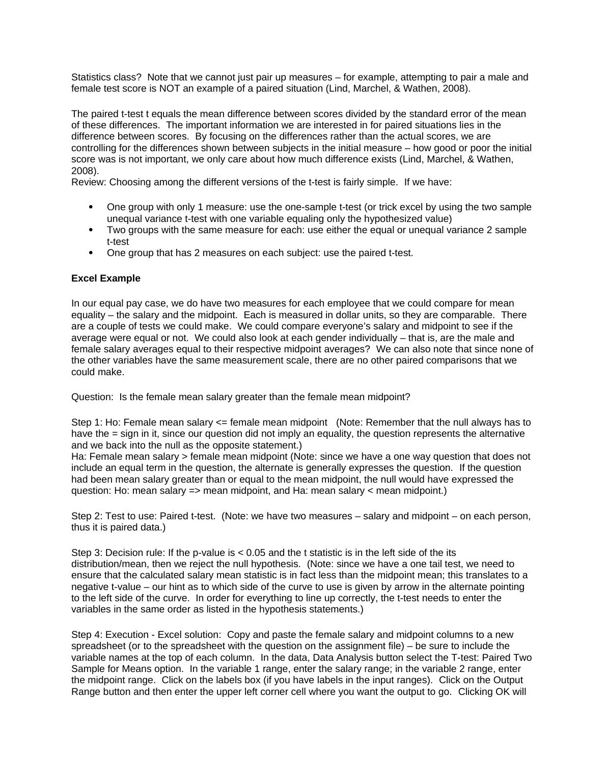
Statistics class? Note that we cannot just pair up measures – for example, attempting to pair a male and female test score is NOT an example of a paired situation (Lind, Marchel, & Wathen, 2008).The paired t-test t equals the mean difference between scores divided by the standard error of the mean of these differences. The important information we are interested in for paired situations lies in the difference between scores. By focusing on the differences rather than the actual scores, we are controlling for the differences shown between subjects in the initial measure – how good or poor the initialscore was is not important, we only care about how much difference exists (Lind, Marchel, & Wathen, 2008).Review: Choosing among the different versions of the t-test is fairly simple. If we have:One group with only 1 measure: use the one-sample t-test (or trick excel by using the two sampleunequal variance t-test with one variable equaling only the hypothesized value)Two groups with the same measure for each: use either the equal or unequal variance 2 sample t-test One group that has 2 measures on each subject: use the paired t-test.Excel ExampleIn our equal pay case, we do have two measures for each employee that we could compare for mean equality – the salary and the midpoint. Each is measured in dollar units, so they are comparable. There are a couple of tests we could make. We could compare everyone’s salary and midpoint to see if the average were equal or not. We could also look at each gender individually – that is, are the male and female salary averages equal to their respective midpoint averages? We can also note that since none ofthe other variables have the same measurement scale, there are no other paired comparisons that we could make.Question: Is the female mean salary greater than the female mean midpoint?Step 1: Ho: Female mean salary <= female mean midpoint (Note: Remember that the null always has to have the = sign in it, since our question did not imply an equality, the question represents the alternative and we back into the null as the opposite statement.)Ha: Female mean salary > female mean midpoint (Note: since we have a one way question that does not include an equal term in the question, the alternate is generally expresses the question. If the question had been mean salary greater than or equal to the mean midpoint, the null would have expressed the question: Ho: mean salary => mean midpoint, and Ha: mean salary < mean midpoint.)Step 2: Test to use: Paired t-test. (Note: we have two measures – salary and midpoint – on each person, thus it is paired data.)Step 3: Decision rule: If the p-value is < 0.05 and the t statistic is in the left side of the its distribution/mean, then we reject the null hypothesis. (Note: since we have a one tail test, we need to ensure that the calculated salary mean statistic is in fact less than the midpoint mean; this translates to a negative t-value – our hint as to which side of the curve to use is given by arrow in the alternate pointing to the left side of the curve. In order for everything to line up correctly, the t-test needs to enter the variables in the same order as listed in the hypothesis statements.)Step 4: Execution - Excel solution: Copy and paste the female salary and midpoint columns to a new spreadsheet (or to the spreadsheet with the question on the assignment file) – be sure to include the variable names at the top of each column. In the data, Data Analysis button select the T-test: Paired TwoSample for Means option. In the variable 1 range, enter the salary range; in the variable 2 range, enter the midpoint range. Click on the labels box (if you have labels in the input ranges). Click on the Output Range button and then enter the upper left corner cell where you want the output to go. Clicking OK will
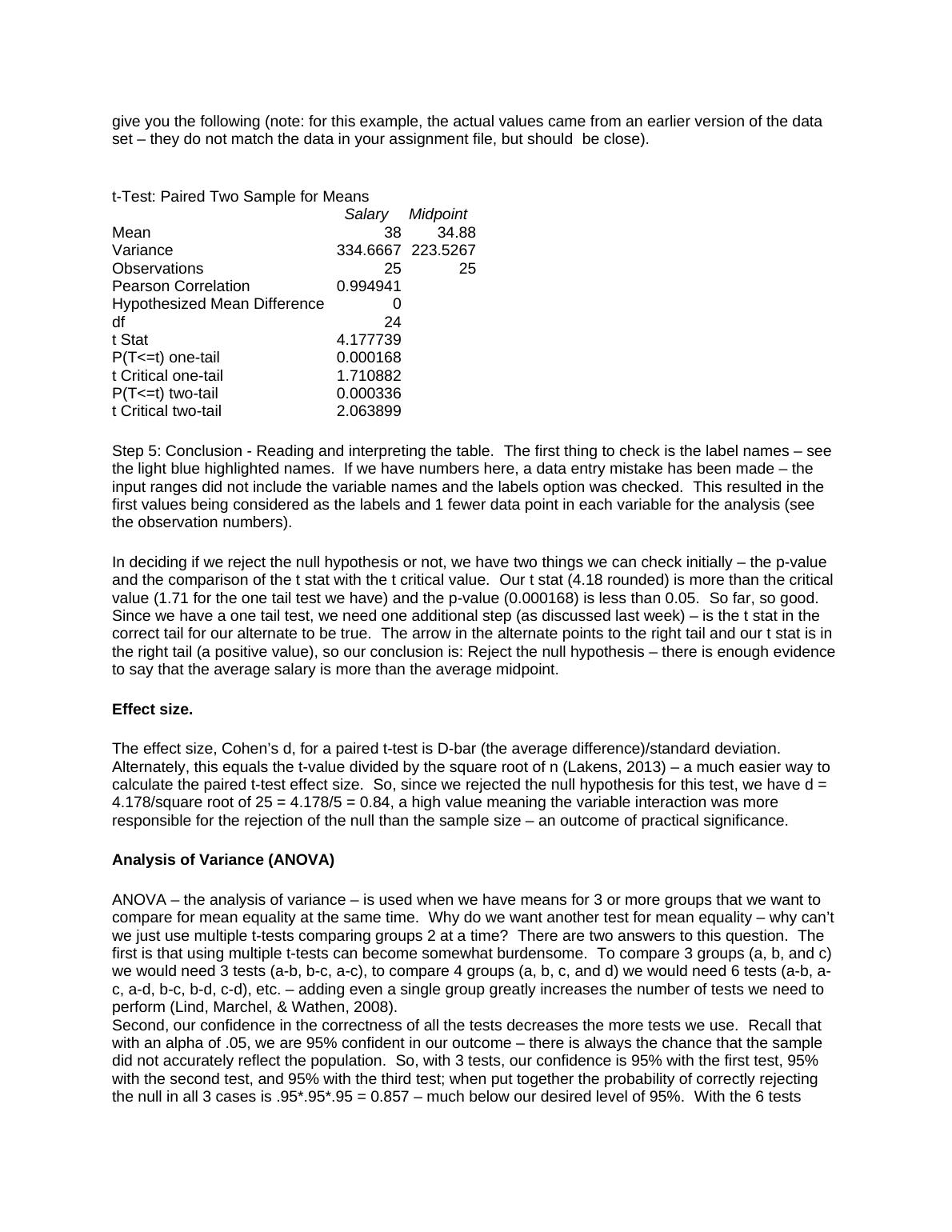
give you the following (note: for this example, the actual values came from an earlier version of the data set – they do not match the data in your assignment file, but should be close).t-Test: Paired Two Sample for Means SalaryMidpointMean3834.88Variance334.6667223.5267Observations2525Pearson Correlation0.994941Hypothesized Mean Difference0df24t Stat4.177739P(T<=t) one-tail0.000168t Critical one-tail1.710882P(T<=t) two-tail0.000336t Critical two-tail2.063899Step 5: Conclusion - Reading and interpreting the table. The first thing to check is the label names – see the light blue highlighted names. If we have numbers here, a data entry mistake has been made – the input ranges did not include the variable names and the labels option was checked. This resulted in the first values being considered as the labels and 1 fewer data point in each variable for the analysis (see the observation numbers).In deciding if we reject the null hypothesis or not, we have two things we can check initially – the p-value and the comparison of the t stat with the t critical value. Our t stat (4.18 rounded) is more than the critical value (1.71 for the one tail test we have) and the p-value (0.000168) is less than 0.05. So far, so good.Since we have a one tail test, we need one additional step (as discussed last week) – is the t stat in the correct tail for our alternate to be true. The arrow in the alternate points to the right tail and our t stat is in the right tail (a positive value), so our conclusion is: Reject the null hypothesis – there is enough evidenceto say that the average salary is more than the average midpoint.Effect size.The effect size, Cohen’s d, for a paired t-test is D-bar (the average difference)/standard deviation.Alternately, this equals the t-value divided by the square root of n (Lakens, 2013) – a much easier way to calculate the paired t-test effect size. So, since we rejected the null hypothesis for this test, we have d = 4.178/square root of 25 = 4.178/5 = 0.84, a high value meaning the variable interaction was more responsible for the rejection of the null than the sample size – an outcome of practical significance.Analysis of Variance (ANOVA)ANOVA – the analysis of variance – is used when we have means for 3 or more groups that we want to compare for mean equality at the same time. Why do we want another test for mean equality – why can’t we just use multiple t-tests comparing groups 2 at a time? There are two answers to this question. The first is that using multiple t-tests can become somewhat burdensome. To compare 3 groups (a, b, and c) we would need 3 tests (a-b, b-c, a-c), to compare 4 groups (a, b, c, and d) we would need 6 tests (a-b, a-c, a-d, b-c, b-d, c-d), etc. – adding even a single group greatly increases the number of tests we need to perform (Lind, Marchel, & Wathen, 2008).Second, our confidence in the correctness of all the tests decreases the more tests we use. Recall that with an alpha of .05, we are 95% confident in our outcome – there is always the chance that the sample did not accurately reflect the population. So, with 3 tests, our confidence is 95% with the first test, 95% with the second test, and 95% with the third test; when put together the probability of correctly rejecting the null in all 3 cases is .95*.95*.95 = 0.857 – much below our desired level of 95%. With the 6 tests
needed for the 4 group comparison, our overall percent becomes 0.735. In order to keep our desired confidence in the results we need to perform all of the comparison in one test – the ANOVA (Lind, Marchel, & Wathen, 2008).ANOVA tests mean equality by comparing the variance of the entire data set with the average variance ofthe individual groups. Therefore, it assumes equal population variances for each group. This assumptionis critical, and should always be verified before using the results of an ANOVA analysis. If you have morethan two groups, compare the largest and smallest variances with the F test (discussed in week 2 for verifying equal variances in choosing the appropriate 2 sample t-test to use) outcome – if they are not significantly different, none of the others will be (Lind, Marchel, & Wathen, 2008).Just how does testing variance equality tell us that means are equal? The underlying logic says that if (1)the groups come from populations having equal variances AND (2) equal means, then the different groups will overlap each other if graphed and the entire data set should have the same mean and variance as each of the samples (within statistical sampling error). If this is true, then the resulting F will be small. If however, the groups have equal variances and UNEQUAL means, they will be spread out rather than overlap and the variance of the overall group will be greater than the average variance for the individual groups and F will be large (Lind, Marchel, & Wathen, 2008).While ANOVA can be used for 2 groups (the results will be identical to those obtained with the two sample equal variance t-test), by convention we use the t for two groups and ANOVA for 3 or more groups (Lind, Marchel, & Wathen, 2008). In our equal pay example, if we think that age is a reason for differing salaries among the grades, we could use ANOVA to see if the average ages for each grade levelare different.ANOVA requires that the different populations being tested have the same variance. This is tested by using the F-test introduced last week. By testing the sample with the largest variance against the sample with the smallest variance, we can see if the variances are statistically equal or not. If the extremes are not significantly different, values between them will also not differ (Lind, Marchel, & Wathen, 2008).Real Life ExampleOne of the course instructors was charged with creating and starting supervisory training classes for a company, The initial proposed 5-day basic supervisory program in a single week met with some initial resistance, as company had never done that before, and the Vice President of Human Resources did not think the managers would accept having their supervisors gone for this period. So, a test was offered.The training would be initially scheduled in 3 different formats, and the managers could pick which they wanted their supervisors to attend – once a week, twice a week, or the full week. At the end, the pre- andpost-test scores – and change in scores - were evaluated to see if format made a difference. The ANOVA was used to verify that the pre-test results were the same – that is, the average knowledge level of supervisors entering the program was not different between the sessions. The paired t-tests showed that learning occurred in each session. At the end, the ANOVA was again used to see if a difference existed between the formats. It did, and this evidence was used to schedule the remainder of the classesin the full 5 day format.Types of ANOVA testsJust as the t-test has 3 versions (one-sample, two-sample, and paired) to choose from, ANOVA also has several choices. The three approaches described in the text match those of the choices that Excel offers – chapter 5’s one way ANVOA is the same as Excel’s ANOVA single factor; chapter 6’s Factorial ANOVA is the same as Excel’s ANOVA: two factor with replication. The authors (Tanner & Youssef-Morgan, 2013) make a somewhat confusing comment on p. 184: “Dependent groups ANOVA is not one of the options Excel offers.” The Excel option 2 factor ANOVA without replication, when used with each example in chapter 7 produce the same results with some additional information – it provides information to test more than the dependent measures across the same subject. We will discuss this in more detail
End of preview
Want to access all the pages? Upload your documents or become a member.
Related Documents
Research Methods for Statistical Analysis - Deskliblg...
|8
|1699
|322
Cognitive Behaviour Therapy PDFlg...
|5
|974
|265