Western Sydney University Statistical Methods in Epidemiology Assignment 2022

Western Sydney University
School of Medicine
Statistical Methods in Epidemiology (401176)
ASSIGNMENT 2
Spring Semester, 2019
Due date: 30 September, 2019
Please answer all questions

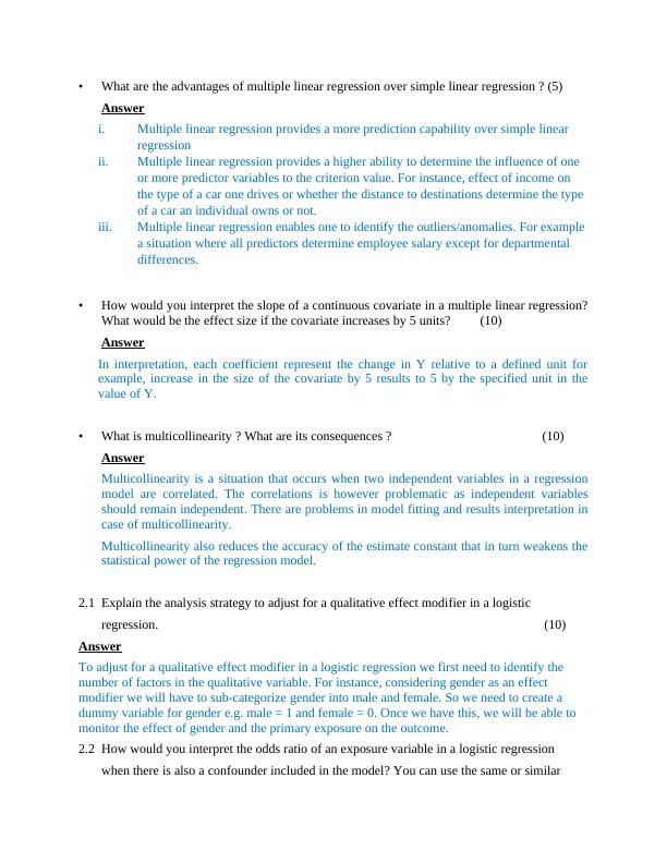
• What are the advantages of multiple linear regression over simple linear regression ? (5)
Answer
i. Multiple linear regression provides a more prediction capability over simple linear
regression
ii. Multiple linear regression provides a higher ability to determine the influence of one
or more predictor variables to the criterion value. For instance, effect of income on
the type of a car one drives or whether the distance to destinations determine the type
of a car an individual owns or not.
iii. Multiple linear regression enables one to identify the outliers/anomalies. For example
a situation where all predictors determine employee salary except for departmental
differences.
• How would you interpret the slope of a continuous covariate in a multiple linear regression?
What would be the effect size if the covariate increases by 5 units? (10)
Answer
In interpretation, each coefficient represent the change in Y relative to a defined unit for
example, increase in the size of the covariate by 5 results to 5 by the specified unit in the
value of Y.
• What is multicollinearity ? What are its consequences ? (10)
Answer
Multicollinearity is a situation that occurs when two independent variables in a regression
model are correlated. The correlations is however problematic as independent variables
should remain independent. There are problems in model fitting and results interpretation in
case of multicollinearity.
Multicollinearity also reduces the accuracy of the estimate constant that in turn weakens the
statistical power of the regression model.
2.1 Explain the analysis strategy to adjust for a qualitative effect modifier in a logistic
regression. (10)
Answer
To adjust for a qualitative effect modifier in a logistic regression we first need to identify the
number of factors in the qualitative variable. For instance, considering gender as an effect
modifier we will have to sub-categorize gender into male and female. So we need to create a
dummy variable for gender e.g. male = 1 and female = 0. Once we have this, we will be able to
monitor the effect of gender and the primary exposure on the outcome.
2.2 How would you interpret the odds ratio of an exposure variable in a logistic regression
when there is also a confounder included in the model? You can use the same or similar

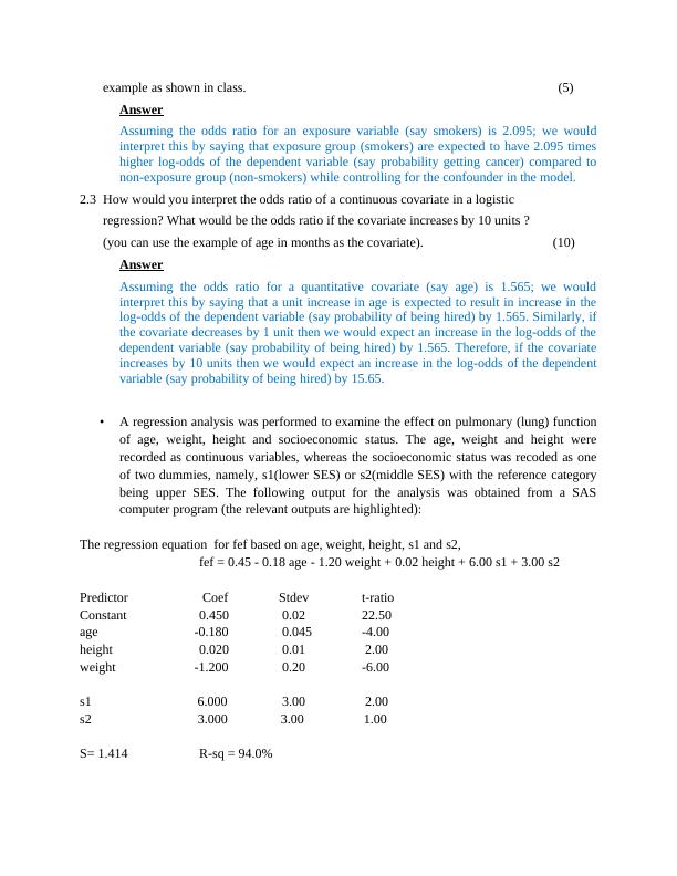
example as shown in class. (5)
Answer
Assuming the odds ratio for an exposure variable (say smokers) is 2.095; we would
interpret this by saying that exposure group (smokers) are expected to have 2.095 times
higher log-odds of the dependent variable (say probability getting cancer) compared to
non-exposure group (non-smokers) while controlling for the confounder in the model.
2.3 How would you interpret the odds ratio of a continuous covariate in a logistic
regression? What would be the odds ratio if the covariate increases by 10 units ?
(you can use the example of age in months as the covariate). (10)
Answer
Assuming the odds ratio for a quantitative covariate (say age) is 1.565; we would
interpret this by saying that a unit increase in age is expected to result in increase in the
log-odds of the dependent variable (say probability of being hired) by 1.565. Similarly, if
the covariate decreases by 1 unit then we would expect an increase in the log-odds of the
dependent variable (say probability of being hired) by 1.565. Therefore, if the covariate
increases by 10 units then we would expect an increase in the log-odds of the dependent
variable (say probability of being hired) by 15.65.
• A regression analysis was performed to examine the effect on pulmonary (lung) function
of age, weight, height and socioeconomic status. The age, weight and height were
recorded as continuous variables, whereas the socioeconomic status was recoded as one
of two dummies, namely, s1(lower SES) or s2(middle SES) with the reference category
being upper SES. The following output for the analysis was obtained from a SAS
computer program (the relevant outputs are highlighted):
The regression equation for fef based on age, weight, height, s1 and s2,
fef = 0.45 - 0.18 age - 1.20 weight + 0.02 height + 6.00 s1 + 3.00 s2
Predictor Coef Stdev t-ratio
Constant 0.450 0.02 22.50
age -0.180 0.045 -4.00
height 0.020 0.01 2.00
weight -1.200 0.20 -6.00
s1 6.000 3.00 2.00
s2 3.000 3.00 1.00
S= 1.414 R-sq = 94.0%

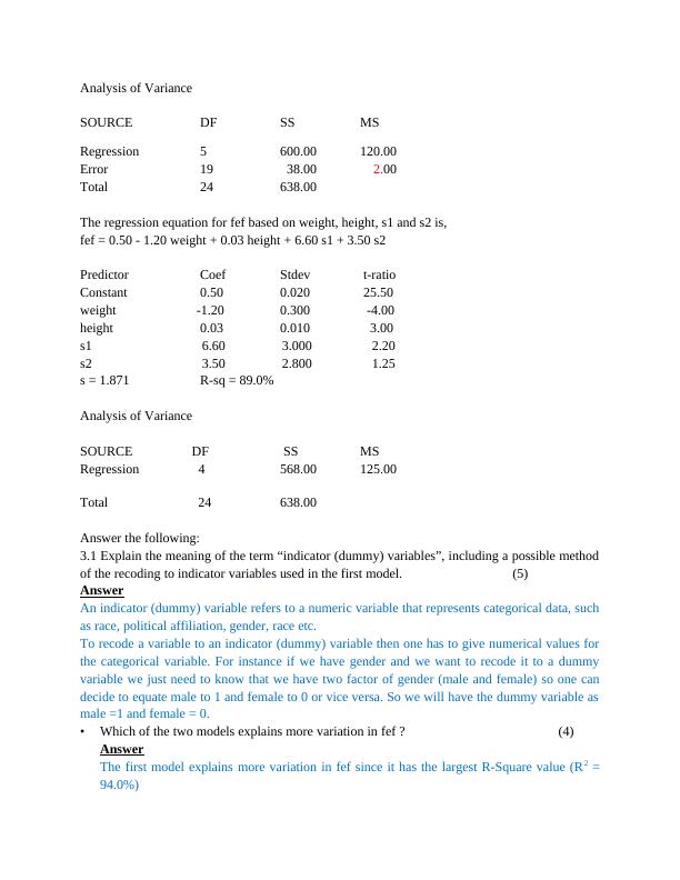
Analysis of Variance
SOURCE DF SS MS
Regression 5 600.00 120.00
Error 19 38.00 2.00
Total 24 638.00
The regression equation for fef based on weight, height, s1 and s2 is,
fef = 0.50 - 1.20 weight + 0.03 height + 6.60 s1 + 3.50 s2
Predictor Coef Stdev t-ratio
Constant 0.50 0.020 25.50
weight -1.20 0.300 -4.00
height 0.03 0.010 3.00
s1 6.60 3.000 2.20
s2 3.50 2.800 1.25
s = 1.871 R-sq = 89.0%
Analysis of Variance
SOURCE DF SS MS
Regression 4 568.00 125.00
Total 24 638.00
Answer the following:
3.1 Explain the meaning of the term “indicator (dummy) variables”, including a possible method
of the recoding to indicator variables used in the first model. (5)
Answer
An indicator (dummy) variable refers to a numeric variable that represents categorical data, such
as race, political affiliation, gender, race etc.
To recode a variable to an indicator (dummy) variable then one has to give numerical values for
the categorical variable. For instance if we have gender and we want to recode it to a dummy
variable we just need to know that we have two factor of gender (male and female) so one can
decide to equate male to 1 and female to 0 or vice versa. So we will have the dummy variable as
male =1 and female = 0.
• Which of the two models explains more variation in fef ? (4)
Answer
The first model explains more variation in fef since it has the largest R-Square value (R2 =
94.0%)