Engineering Mathematics 2 Project: Vehicle Suspension Analysis
VerifiedAdded on 2022/08/16
|5
|2842
|11
Project
AI Summary
This project presents a comprehensive analysis of a vehicle suspension system, modeled as a mass-spring-damper system, utilizing Newtonian mechanics and mathematical methods. The study employs differential equations, transfer functions, and state-space modeling to characterize the system's behavior. Stability analysis and the determination of critical suspension parameters, such as natural frequency and damping ratio, are conducted using mathematical expressions and MATLAB simulations. The project investigates the effects of varying spring stiffness and damping ratios on system performance, including transient and frequency response analyses using Bode plots and step responses. Furthermore, the project simulates the vehicle's response to different road surface conditions, incorporating sinusoidal and cosine functions to represent road unevenness. The design process involves selecting appropriate parameters to meet specified performance criteria, and the results are presented through simulations and state-space model analysis, concluding with an evaluation of the system's stability and performance under various conditions. The project aims to provide a practical understanding of vehicle suspension system design and analysis.
Engineering Mathematics 2
1st Author
1st author's affiliation
1st line of address
2nd line of address
Telephone number, incl. country code
1st author's E-mail address
2nd Author
2nd author's affiliation
1st line of address
2nd line of address
Telephone number, incl. country code
2nd E-mail
3rd Author
3rd author's affiliation
1st line of address
2nd line of address
Telephone number, incl. country code
3rd E-mail
ABSTRACT
In this project, a general analysis of vehicle suspension system is
produced with the help of Newtonian mechanics and
mathematical methods. The suspension system is assumed to
follow the behavior of mass-spring-damper system approximately.
Thus the system is analyzed with transfer function and state space
modelling common for mass-spring-damper and stability of
system along with its critical suspension parameters are measured
with suitable mathematical expressions and simulations in
MATLAB.
1. INTRODUCTION
The vehicle suspension system is an important part of a car which
helps to minimize the discomfort of travelling in non-smooth
surfaces. Basically the suspension system works as a low pass
filter which helps to filter out the high frequency oscillations
caused by irregular road surfaces and thus to maintain stability of
vehicle while moving. The main parameters of vehicle suspension
are the stiffness constant and viscosity constant of the damper
which corresponds to various suspension equipment in actual
vehicle [1]. An inaccurate choice of the parameters can result in
poor vehicle performance and may be sometimes sudden failure
while moving that can cause accidents due to lack of control over
the vehicle. In this study these parameters of suspension suitable
for a fixed vehicle mass is estimated by using Newton’s law of
mechanics with differential equation and stability analysis of
control system. The vehicle is simulated for different values of
these parameters and the critical natural frequency and damping
ratio of the system is estimated which is very much important for
the vehicle dynamics [2].
2. DEVELOPMENT OF SYSTEM
MODEL & ANALYSIS OF SYSTEM
CHARACTERISTICS
There are four forces acting on the system which are force due to
gravity, force for spring, damping force and net external forces
F(t). Now, force due to gravity is
Fg = mg
Now, spring force can be modelled by Hooke’s law that states
force exerted by spring is proportional to displacement from its
natural length and here the natural length is spring length L added
with relative displacement between car and the road [4].
Hence, Fs = -k(L + (u(t)- y(t)))
Now, the damping force or the car’s suspension responds to
relative velocity between car and road unevenness and given by,
Fd = -c(u’(t)-y’(t))
Now, by putting all of the forces together and applying newton’s
second law which gives acceleration of an object is equal to all the
forces applied to it gives,
mu’’(t) = mg – k(L+u(t) – y(t)) -c(u’(t)-y’(t)) + F(t)
Or, mu’’(t) + c(u’(t)-y’(t)) + k(u(t) – y(t)) = mg – kL + F(t)
Paraphrase This Document
Need a fresh take? Get an instant paraphrase of this document with our AI Paraphraser
2.1 Differential equation of system:
Now, when the car is at rest then gravitational force and spring
force cancels each other. Thus the differential equation of the
system can be represented by the following equation
mu’’(t) + c(u’(t)-y’(t)) + k(u(t)-y(t)) = F(t) (1)
Here, m = mass of the car.
u’’ = acceleration of the car.
u’ = car velocity
y’ = change of road unevenness
u = car displacement
y = road unevenness displacement
F(t) = external force applied to the system
It can be seen from the equation that highest order of the
differential equation is two and hence it is a 2nd order differential
equation [5]. In the equation the driving force is the external force
applied to the system, the spring or compression/extension
component of the suspension represents the restoring force and
the damper of suspension is the energy absorbing force.
2.2 Applied simplifications on system
Now, in the system it is assumed that the driving, restoring force
and the energy absorbing corresponds to external force, spring and
a damper, however, in actual case of a car the forces can be much
complicated [3]. As there can be several external forces can be
acting on the car and may not vary only according to time. Also,
the restoring force is real case is not exactly corresponds to the
behavior of a spring, additional equipment like gears or others
may exist. The damping force that absorbs energy while the car is
moving through rough surfaces often is of non-linear type,
however, in the model a linear constant is multiplied with the
damping force [6]. Thus more complicated mathematical equation
is needed to model the car suspension system such that better
behavior of its dynamics can be obtained matching with real
cases.
2.3 Natural frequency and damping ratio
The natural frequency of the system is expressed by the
coefficients of the differential equation as given by,
ωn = √k /m and the damping ratio ξ= c
2 √km
Here, k = spring stiffness, c = damper viscosity and m = mass
Now, when the system is in equilibrium then no external force is
applied to the system and hence F(t) = 0 [8]. Now the differential
equation in terms these parameter becomes
( 1
ωn
2 ) u ’ ’ ( t ) + ( 2ξ
ωn ) (u ¿¿ ' ( t ) − y ' (t))+(u (t)− y (t ))=0 ¿
2.4 Transfer function of system
The transfer function of the system is obtained by taking forward
Laplace transform of the equation (1) assuming zero initial
conditions i.e. u(0) = 0 and u’(0) = 0.
ms^2U(s) + csU(s) – csY(s) + kU(s) – kY(s) = 0
U(s)(ms^2 + cs + k) = (cs+k)Y(s)
U(s)/Y(s) = (cs+k)/(ms^2 + cs + k)
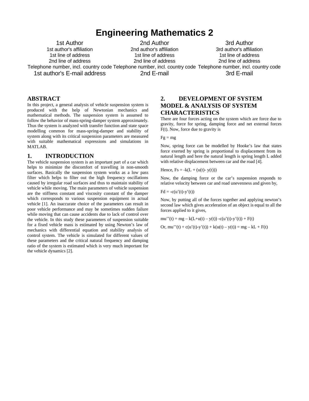
Now, the system characteristics is investigated for different values
of k and ξ with a fixed mass of 750 kg as provided for the
assignment. The damping coefficient c can be determined from
the expression of ξ as
c=2ξ √ km
2.5 Transient and frequency analysis for
different spring stiffness (k) and damping
ratio (ξ)
Now, frequency domain analysis of the system is first performed
by loading the system transfer function MATLAB. The bode plot
is an appropriate frequency domain analysis which is obtained in
MATLAB as shown in Figure 1.
The different values of k are 7.5*10^3, 7.5*10^4 and 7.5*10^5
N/m respectively and different values of ξ are 0.15, 0.3 and 0.6.
The transfer functions are obtained in MATLAB are
Sys 1= 711.5 s +7500
750 s2+711.5 s+7500
Sys 2= 4500 s+75000
750 s2+ 4500 s +75000
Sys 3= 2.846e4 s +750000
750 s2 +2.846e4 s+750000
From the bode plots it is found that the gain margin and phase
margins are always positive for all value spring coefficients (k).
Hence, it can be concluded that the open loop system is
asymptotically stable with finite gain crossover frequency.
However, the open loop system has infinite gain margin indicating
no finite phase crossovers [6].
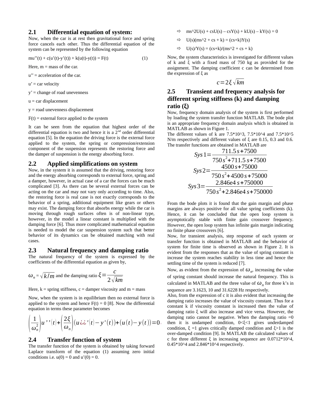
Now, for transient analysis, step response of each system or
transfer function is obtained in MATLAB and the behavior of
system for finite time is observed as shown in Figure 2. It is
evident from the responses that as the value of spring constant is
increase the system reaches stability in less time and hence the
settling time of the system is reduced [7].
Now, as evident from the expression of ωn, increasing the value
of spring constant should increase the natural frequency. This is
calculated in MATLAB and the three value of ωn for three k’s in
sequence are 3.1623, 10 and 31.6228 Hz respectively.
Also, from the expression of c it is also evident that increasing the
damping ratio increases the value of viscosity constant. Thus for a
constant k if viscosity constant is increased then the value of
damping ratio ξ will also increase and vice versa. However, the
damping ratio cannot be negative. When the damping ratio =0
then it is undamped condition, 0<ξ<1 gives underdamped
condition, ξ =1 gives critically damped condition and ξ>1 is the
over-damped condition [9]. In MATLAB the calculated values of
c for three different ξ in increasing sequence are 0.0712*10^4,
0.45*10^4 and 2.846*10^4 respectively.
Now, when the car is at rest then gravitational force and spring
force cancels each other. Thus the differential equation of the
system can be represented by the following equation
mu’’(t) + c(u’(t)-y’(t)) + k(u(t)-y(t)) = F(t) (1)
Here, m = mass of the car.
u’’ = acceleration of the car.
u’ = car velocity
y’ = change of road unevenness
u = car displacement
y = road unevenness displacement
F(t) = external force applied to the system
It can be seen from the equation that highest order of the
differential equation is two and hence it is a 2nd order differential
equation [5]. In the equation the driving force is the external force
applied to the system, the spring or compression/extension
component of the suspension represents the restoring force and
the damper of suspension is the energy absorbing force.
2.2 Applied simplifications on system
Now, in the system it is assumed that the driving, restoring force
and the energy absorbing corresponds to external force, spring and
a damper, however, in actual case of a car the forces can be much
complicated [3]. As there can be several external forces can be
acting on the car and may not vary only according to time. Also,
the restoring force is real case is not exactly corresponds to the
behavior of a spring, additional equipment like gears or others
may exist. The damping force that absorbs energy while the car is
moving through rough surfaces often is of non-linear type,
however, in the model a linear constant is multiplied with the
damping force [6]. Thus more complicated mathematical equation
is needed to model the car suspension system such that better
behavior of its dynamics can be obtained matching with real
cases.
2.3 Natural frequency and damping ratio
The natural frequency of the system is expressed by the
coefficients of the differential equation as given by,
ωn = √k /m and the damping ratio ξ= c
2 √km
Here, k = spring stiffness, c = damper viscosity and m = mass
Now, when the system is in equilibrium then no external force is
applied to the system and hence F(t) = 0 [8]. Now the differential
equation in terms these parameter becomes
( 1
ωn
2 ) u ’ ’ ( t ) + ( 2ξ
ωn ) (u ¿¿ ' ( t ) − y ' (t))+(u (t)− y (t ))=0 ¿
2.4 Transfer function of system
The transfer function of the system is obtained by taking forward
Laplace transform of the equation (1) assuming zero initial
conditions i.e. u(0) = 0 and u’(0) = 0.
ms^2U(s) + csU(s) – csY(s) + kU(s) – kY(s) = 0
U(s)(ms^2 + cs + k) = (cs+k)Y(s)
U(s)/Y(s) = (cs+k)/(ms^2 + cs + k)
Now, the system characteristics is investigated for different values
of k and ξ with a fixed mass of 750 kg as provided for the
assignment. The damping coefficient c can be determined from
the expression of ξ as
c=2ξ √ km
2.5 Transient and frequency analysis for
different spring stiffness (k) and damping
ratio (ξ)
Now, frequency domain analysis of the system is first performed
by loading the system transfer function MATLAB. The bode plot
is an appropriate frequency domain analysis which is obtained in
MATLAB as shown in Figure 1.
The different values of k are 7.5*10^3, 7.5*10^4 and 7.5*10^5
N/m respectively and different values of ξ are 0.15, 0.3 and 0.6.
The transfer functions are obtained in MATLAB are
Sys 1= 711.5 s +7500
750 s2+711.5 s+7500
Sys 2= 4500 s+75000
750 s2+ 4500 s +75000
Sys 3= 2.846e4 s +750000
750 s2 +2.846e4 s+750000
From the bode plots it is found that the gain margin and phase
margins are always positive for all value spring coefficients (k).
Hence, it can be concluded that the open loop system is
asymptotically stable with finite gain crossover frequency.
However, the open loop system has infinite gain margin indicating
no finite phase crossovers [6].
Now, for transient analysis, step response of each system or
transfer function is obtained in MATLAB and the behavior of
system for finite time is observed as shown in Figure 2. It is
evident from the responses that as the value of spring constant is
increase the system reaches stability in less time and hence the
settling time of the system is reduced [7].
Now, as evident from the expression of ωn, increasing the value
of spring constant should increase the natural frequency. This is
calculated in MATLAB and the three value of ωn for three k’s in
sequence are 3.1623, 10 and 31.6228 Hz respectively.
Also, from the expression of c it is also evident that increasing the
damping ratio increases the value of viscosity constant. Thus for a
constant k if viscosity constant is increased then the value of
damping ratio ξ will also increase and vice versa. However, the
damping ratio cannot be negative. When the damping ratio =0
then it is undamped condition, 0<ξ<1 gives underdamped
condition, ξ =1 gives critically damped condition and ξ>1 is the
over-damped condition [9]. In MATLAB the calculated values of
c for three different ξ in increasing sequence are 0.0712*10^4,
0.45*10^4 and 2.846*10^4 respectively.
3. Analysis of shock absorber over a
simulated road surface
3.1 Simulation of road surface
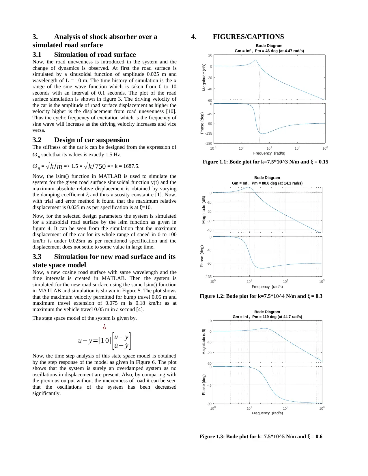
Now, the road unevenness is introduced in the system and the
change of dynamics is observed. At first the road surface is
simulated by a sinusoidal function of amplitude 0.025 m and
wavelength of L = 10 m. The time history of simulation is the x
range of the sine wave function which is taken from 0 to 10
seconds with an interval of 0.1 seconds. The plot of the road
surface simulation is shown in figure 3. The driving velocity of
the car is the amplitude of road surface displacement as higher the
velocity higher is the displacement from road unevenness [10].
Thus the cyclic frequency of excitation which is the frequency of
sine wave will increase as the driving velocity increases and vice
versa.
3.2 Design of car suspension
The stiffness of the car k can be designed from the expression of
ωn such that its values is exactly 1.5 Hz.
ωn = √k /m => 1.5 = √k /750 => k = 1687.5.
Now, the lsim() function in MATLAB is used to simulate the
system for the given road surface sinusoidal function y(t) and the
maximum absolute relative displacement is obtained by varying
the damping coefficient ξ and thus viscosity constant c [1]. Now,
with trial and error method it found that the maximum relative
displacement is 0.025 m as per specification is at ξ=10.
Now, for the selected design parameters the system is simulated
for a sinusoidal road surface by the lsim function as given in
figure 4. It can be seen from the simulation that the maximum
displacement of the car for its whole range of speed in 0 to 100
km/hr is under 0.025m as per mentioned specification and the
displacement does not settle to some value in large time.
3.3 Simulation for new road surface and its
state space model
Now, a new cosine road surface with same wavelength and the
time intervals is created in MATLAB. Then the system is
simulated for the new road surface using the same lsim() function
in MATLAB and simulation is shown in Figure 5. The plot shows
that the maximum velocity permitted for bump travel 0.05 m and
maximum travel extension of 0.075 m is 0.18 km/hr as at
maximum the vehicle travel 0.05 m in a second [4].
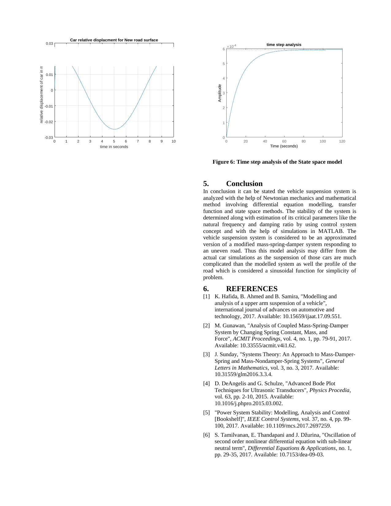
The state space model of the system is given by,
¿
u− y=[1 0] [ u− y
˙u− ˙y ]
Now, the time step analysis of this state space model is obtained
by the step response of the model as given in Figure 6. The plot
shows that the system is surely an overdamped system as no
oscillations in displacement are present. Also, by comparing with
the previous output without the unevenness of road it can be seen
that the oscillations of the system has been decreased
significantly.
4. FIGURES/CAPTIONS
-60
-40
-20
0
20
Magnitude (dB)
10 -1 10 0 10 1 10 2 103
-180
-135
-90
-45
0
Phase (deg)
Bode Diagram
Gm = Inf , Pm = 46 deg (at 4.47 rad/s)
Frequency (rad/s)
-40
-30
-20
-10
0
Magnitude (dB)
10 0 101 102 10 3
-135
-90
-45
0
Phase (deg)
Bode Diagram
Gm = Inf , Pm = 80.6 deg (at 14.1 rad/s)
Frequency (rad/s)
-30
-20
-10
0
10
Magnitude (dB)
100 101 102 103
-90
-45
0
Phase (deg)
Bode Diagram
Gm = Inf , Pm = 119 deg (at 44.7 rad/s)
Frequency (rad/s)
Figure 1.1: Bode plot for k=7.5*10^3 N/m and ξ = 0.15
Figure 1.2: Bode plot for k=7.5*10^4 N/m and ξ = 0.3
Figure 1.3: Bode plot for k=7.5*10^5 N/m and ξ = 0.6
simulated road surface
3.1 Simulation of road surface
Now, the road unevenness is introduced in the system and the
change of dynamics is observed. At first the road surface is
simulated by a sinusoidal function of amplitude 0.025 m and
wavelength of L = 10 m. The time history of simulation is the x
range of the sine wave function which is taken from 0 to 10
seconds with an interval of 0.1 seconds. The plot of the road
surface simulation is shown in figure 3. The driving velocity of
the car is the amplitude of road surface displacement as higher the
velocity higher is the displacement from road unevenness [10].
Thus the cyclic frequency of excitation which is the frequency of
sine wave will increase as the driving velocity increases and vice
versa.
3.2 Design of car suspension
The stiffness of the car k can be designed from the expression of
ωn such that its values is exactly 1.5 Hz.
ωn = √k /m => 1.5 = √k /750 => k = 1687.5.
Now, the lsim() function in MATLAB is used to simulate the
system for the given road surface sinusoidal function y(t) and the
maximum absolute relative displacement is obtained by varying
the damping coefficient ξ and thus viscosity constant c [1]. Now,
with trial and error method it found that the maximum relative
displacement is 0.025 m as per specification is at ξ=10.
Now, for the selected design parameters the system is simulated
for a sinusoidal road surface by the lsim function as given in
figure 4. It can be seen from the simulation that the maximum
displacement of the car for its whole range of speed in 0 to 100
km/hr is under 0.025m as per mentioned specification and the
displacement does not settle to some value in large time.
3.3 Simulation for new road surface and its
state space model
Now, a new cosine road surface with same wavelength and the
time intervals is created in MATLAB. Then the system is
simulated for the new road surface using the same lsim() function
in MATLAB and simulation is shown in Figure 5. The plot shows
that the maximum velocity permitted for bump travel 0.05 m and
maximum travel extension of 0.075 m is 0.18 km/hr as at
maximum the vehicle travel 0.05 m in a second [4].
The state space model of the system is given by,
¿
u− y=[1 0] [ u− y
˙u− ˙y ]
Now, the time step analysis of this state space model is obtained
by the step response of the model as given in Figure 6. The plot
shows that the system is surely an overdamped system as no
oscillations in displacement are present. Also, by comparing with
the previous output without the unevenness of road it can be seen
that the oscillations of the system has been decreased
significantly.
4. FIGURES/CAPTIONS
-60
-40
-20
0
20
Magnitude (dB)
10 -1 10 0 10 1 10 2 103
-180
-135
-90
-45
0
Phase (deg)
Bode Diagram
Gm = Inf , Pm = 46 deg (at 4.47 rad/s)
Frequency (rad/s)
-40
-30
-20
-10
0
Magnitude (dB)
10 0 101 102 10 3
-135
-90
-45
0
Phase (deg)
Bode Diagram
Gm = Inf , Pm = 80.6 deg (at 14.1 rad/s)
Frequency (rad/s)
-30
-20
-10
0
10
Magnitude (dB)
100 101 102 103
-90
-45
0
Phase (deg)
Bode Diagram
Gm = Inf , Pm = 119 deg (at 44.7 rad/s)
Frequency (rad/s)
Figure 1.1: Bode plot for k=7.5*10^3 N/m and ξ = 0.15
Figure 1.2: Bode plot for k=7.5*10^4 N/m and ξ = 0.3
Figure 1.3: Bode plot for k=7.5*10^5 N/m and ξ = 0.6
⊘ This is a preview!⊘
Do you want full access?
Subscribe today to unlock all pages.
Trusted by 1+ million students worldwide
0 2 4 6 8 10 12
0
0.2
0.4
0.6
0.8
1
1.2
1.4
1.6
1.8
Step Response
Time (seconds)
Amplitude
0 0.2 0.4 0.6 0.8 1 1.2 1.4 1.6 1.8
0
0.5
1
1.5
Step Response
Time (seconds)
Amplitude
0 0.05 0.1 0.15 0.2 0.25 0.3 0.35
0
0.2
0.4
0.6
0.8
1
1.2
1.4
Step Response
Time (seconds)
Amplitude
0 1 2 3 4 5 6 7 8 9 10
Time in secs
-0.05
-0.04
-0.03
-0.02
-0.01
0
0.01
0.02
0.03
0.04
0.05
Road surface displacment in meters
Simulation of road surface
0 1 2 3 4 5 6 7 8 9 10
time in seconds
-0.03
-0.02
-0.01
0
0.01
0.02
0.03
relative displacement of car in meters
Car relative displacment for given design paramters
Figure 2.1: transient step response for k=7.5*10^3 N/m
Figure 2.2: transient step response for k=7.5*10^4 N/m
Figure 2.3: transient step response for k=7.5*10^5 N/m
and ξ = 0.6
Figure 4: Simulation of car for Sinusoidal road
0
0.2
0.4
0.6
0.8
1
1.2
1.4
1.6
1.8
Step Response
Time (seconds)
Amplitude
0 0.2 0.4 0.6 0.8 1 1.2 1.4 1.6 1.8
0
0.5
1
1.5
Step Response
Time (seconds)
Amplitude
0 0.05 0.1 0.15 0.2 0.25 0.3 0.35
0
0.2
0.4
0.6
0.8
1
1.2
1.4
Step Response
Time (seconds)
Amplitude
0 1 2 3 4 5 6 7 8 9 10
Time in secs
-0.05
-0.04
-0.03
-0.02
-0.01
0
0.01
0.02
0.03
0.04
0.05
Road surface displacment in meters
Simulation of road surface
0 1 2 3 4 5 6 7 8 9 10
time in seconds
-0.03
-0.02
-0.01
0
0.01
0.02
0.03
relative displacement of car in meters
Car relative displacment for given design paramters
Figure 2.1: transient step response for k=7.5*10^3 N/m
Figure 2.2: transient step response for k=7.5*10^4 N/m
Figure 2.3: transient step response for k=7.5*10^5 N/m
and ξ = 0.6
Figure 4: Simulation of car for Sinusoidal road
Paraphrase This Document
Need a fresh take? Get an instant paraphrase of this document with our AI Paraphraser
0 1 2 3 4 5 6 7 8 9 10
time in seconds
-0.03
-0.02
-0.01
0
0.01
0.02
0.03
relative displacement of car in meters
Car relative displacment for New road surface
0 20 40 60 80 100 120
0
1
2
3
4
5
6 10-4 time step analysis
Time (seconds)
Amplitude
5. Conclusion
In conclusion it can be stated the vehicle suspension system is
analyzed with the help of Newtonian mechanics and mathematical
method involving differential equation modelling, transfer
function and state space methods. The stability of the system is
determined along with estimation of its critical parameters like the
natural frequency and damping ratio by using control system
concept and with the help of simulations in MATLAB. The
vehicle suspension system is considered to be an approximated
version of a modified mass-spring-damper system responding to
an uneven road. Thus this model analysis may differ from the
actual car simulations as the suspension of those cars are much
complicated than the modelled system as well the profile of the
road which is considered a sinusoidal function for simplicity of
problem.
6. REFERENCES
[1] K. Hafida, B. Ahmed and B. Samira, "Modelling and
analysis of a upper arm suspension of a vehicle",
international journal of advances on automotive and
technology, 2017. Available: 10.15659/ijaat.17.09.551.
[2] M. Gunawan, "Analysis of Coupled Mass-Spring-Damper
System by Changing Spring Constant, Mass, and
Force", ACMIT Proceedings, vol. 4, no. 1, pp. 79-91, 2017.
Available: 10.33555/acmit.v4i1.62.
[3] J. Sunday, "Systems Theory: An Approach to Mass-Damper-
Spring and Mass-Nondamper-Spring Systems", General
Letters in Mathematics, vol. 3, no. 3, 2017. Available:
10.31559/glm2016.3.3.4.
[4] D. DeAngelis and G. Schulze, "Advanced Bode Plot
Techniques for Ultrasonic Transducers", Physics Procedia,
vol. 63, pp. 2-10, 2015. Available:
10.1016/j.phpro.2015.03.002.
[5] "Power System Stability: Modelling, Analysis and Control
[Bookshelf]", IEEE Control Systems, vol. 37, no. 4, pp. 99-
100, 2017. Available: 10.1109/mcs.2017.2697259.
[6] S. Tamilvanan, E. Thandapani and J. Džurina, "Oscillation of
second order nonlinear differential equation with sub-linear
neutral term", Differential Equations & Applications, no. 1,
pp. 29-35, 2017. Available: 10.7153/dea-09-03.
Figure 6: Time step analysis of the State space model
1 out of 5

Your All-in-One AI-Powered Toolkit for Academic Success.
+13062052269
info@desklib.com
Available 24*7 on WhatsApp / Email
![[object Object]](/_next/static/media/star-bottom.7253800d.svg)
Unlock your academic potential
Copyright © 2020–2026 A2Z Services. All Rights Reserved. Developed and managed by ZUCOL.